Late Chunking in Long-Context Embedding Models
Chunking long documents while preserving contextual information is challenging. We introduce the "Late Chunking" that leverages long-context embedding models to generate contextual chunk embeddings for better retrieval applications.


About a year ago, in October 2023, we released the world's first open-source embedding model with an 8K context length, jina-embeddings-v2-base-en. Since then, there has been quite some debate about the usefulness of long-context in embedding models. For many applications, encoding a document thousands of words long into a single embedding representation is not ideal. Many use cases require retrieving smaller portions of the text, and dense vector-based retrieval systems often perform better with smaller text segments, as the semantics are less likely to be "over-compressed" in the embedding vectors.
Retrieval-Augmented Generation (RAG) is one of the most well-known applications that requires splitting documents into smaller text chunks (say within 512 tokens). These chunks are usually stored in a vector database, with vector representations generated by a text embedding model. During runtime, the same embedding model encodes a query into a vector representation, which is then used to identify relevant stored text chunks. These chunks are subsequently passed to a large language model (LLM), which synthesizes a response to the query based on the retrieved texts.

In short, embedding smaller chunks seems to be more preferable, partly due to the limited input sizes of downstream LLMs, but also because there’s a concern that important contextual information in a long context may get diluted when compressed into a single vector.
But if the industry only ever needs embedding models with a 512-context length, what’s the point of training models with an 8192-context length at all?
In this article, we revisit this important, albeit uncomfortable, question by exploring the limitations of the naive chunking-embedding pipeline in RAG. We introduce a new approach called "Late Chunking," which leverages the rich contextual information provided by 8192-length embedding models to more effectively embed chunks.
The Lost Context Problem
The simple RAG pipeline of chunking-embedding-retrieving-generating is not without its challenges. Specifically, this process can destroy long-distance contextual dependencies. In other words, when relevant information is spread across multiple chunks, taking text segments out of context can render them ineffective, making this approach particularly problematic.
In the image below, a Wikipedia article is split into chunks of sentences. You can see that phrases like "its" and "the city" reference "Berlin," which is mentioned only in the first sentence. This makes it harder for the embedding model to link these references to the correct entity, thereby producing a lower-quality vector representation.
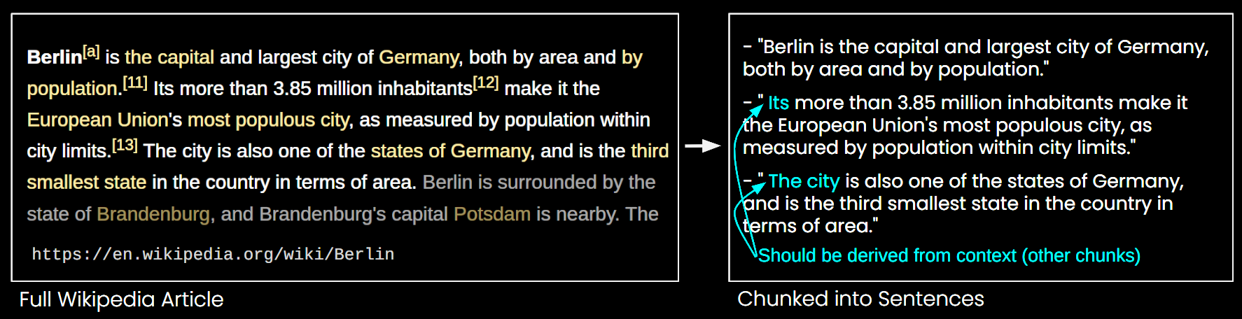
This means, if we split a long article into sentence-length chunks, as in the example above, a RAG system might struggle to answer a query like "What is the population of Berlin?" Because the city name and the population never appear together in a single chunk, and without any larger document context, an LLM presented with one of these chunks cannot resolve anaphoric references like "it" or "the city."
There are some heuristics to alleviate this issue, such as resampling with a sliding window, using multiple context window lengths, and performing multi-pass document scans. However, like all heuristics, these approaches are hit-or-miss; they may work in some cases, but there's no theoretical guarantee of their effectiveness.
The Solution: Late Chunking
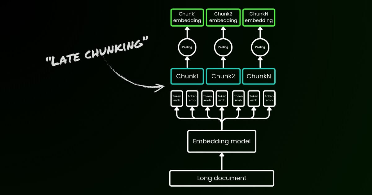
The naive encoding approach (as seen on the left side of the image below) involves using sentences, paragraphs, or maximum length limits to split the text a priori. Afterward, an embedding model is repetitively applied to these resulting chunks. To generate a single embedding for each chunk, many embedding models use mean pooling on these token-level embeddings to output a single embedding vector.

In contrast, the "Late Chunking" approach we propose in this article first applies the transformer layer of the embedding model to the entire text or as much of it as possible. This generates a sequence of vector representations for each token that encompasses textual information from the entire text. Subsequently, mean pooling is applied to each chunk of this sequence of token vectors, yielding embeddings for each chunk that consider the entire text's context. Unlike the naive encoding approach, which generates independent and identically distributed (i.i.d.) chunk embeddings, late chunking creates a set of chunk embeddings where each one is "conditioned on" the previous ones, thereby encoding more contextual information for each chunk.
Obviously to effectively apply late chunking, we need long-context embedding models like jina-embeddings-v2-base-en, which support up to 8192 tokens—roughly ten standard pages of text. Text segments of this size are much less likely to have contextual dependencies that require an even longer context to resolve.
It's important to highlight that late chunking still requires boundary cues, but these cues are used only after obtaining the token-level embeddings—hence the term "late" in its naming.
| Naive Chunking | Late Chunking | |
|---|---|---|
| The need of boundary cues | Yes | Yes |
| The use of boundary cues | Directly in preprocessing | After getting the token-level embeddings from the transformer layer |
| The resulting chunk embeddings | i.i.d. | Conditional |
| Contextual information of nearby chunks | Lost. Some heuristics (like overlap sampling) to alleviate this | Well-preserved by long-context embedding models |
Implementation and Qualitative Evaluation


The implementation of late chunking can be found in the Google Colab linked above. Here, we utilize our recent feature release in the Tokenizer API, which leverages all possible boundary cues to segment a long document into meaningful chunks. More discussion on the algorithm behind this feature can be found on X.
Based. Semantic chunking is overrated. Especially when you write a super regex that leverages all possible boundary cues and heuristics to segment text accurately without the need for complex language models. Just think about the speed and the hosting cost. This 50-line,… pic.twitter.com/AtBCSrn7nI
— Jina AI (@JinaAI_) August 14, 2024
When applying late chunking to the Wikipedia example above, you can immediately see an improvement in semantic similarity. For instance, in the case of "the city" and "Berlin" within a Wikipedia article, the vectors representing "the city" now contain information linking it to the previous mention of "Berlin," making it a much better match for queries involving that city name.
| Query | Chunk | Sim. on naive chunking | Sim. on late chunking |
|---|---|---|---|
| Berlin | Berlin is the capital and largest city of Germany, both by area and by population. | 0.849 | 0.850 |
| Berlin | Its more than 3.85 million inhabitants make it the European Union's most populous city, as measured by population within city limits. | 0.708 | 0.825 |
| Berlin | The city is also one of the states of Germany, and is the third smallest state in the country in terms of area. | 0.753 | 0.850 |
You can observe this in the numerical results above, which compare the embedding of the term "Berlin" to various sentences from the article about Berlin using cosine similarity. The column "Sim. on IID chunk embeddings" shows the similarity values between the query embedding of "Berlin" and the embeddings using a priori chunking, while "Sim. under contextual chunk embedding" represents the results with late chunking method.
Quantitative Evaluation on BEIR
To verify the effectiveness of late chunking beyond a toy example, we tested it using some of the retrieval benchmarks from BeIR. These retrieval tasks consist of a query set, a corpus of text documents, and a QRels file that stores information about the IDs of documents relevant to each query.
To identify the relevant documents for a query, the documents are chunked, encoded into an embedding index, and the most similar chunks are determined for each query embedding using k-nearest neighbors (kNN). Since each chunk corresponds to a document, the kNN ranking of chunks can be converted into a kNN ranking of documents (retaining only the first occurrence for documents appearing multiple times in the ranking). This resulting ranking is then compared to the ranking provided by the ground-truth QRels file, and retrieval metrics like nDCG@10 are calculated. This procedure is depicted below, and the evaluation script can be found in this repository for reproducibility.
 jina-ai
We ran this evaluation on various BeIR datasets, comparing naive chunking with our late chunking method. For getting the boundary cues, we used a regex that splits the texts into strings of roughly 256 tokens. Both the naive and late chunking evaluation used jina-embeddings-v2-small-en as the embedding model; a smaller version of the v2-base-en model that still supports up to 8192-token length. Results can be found in the table below.
| Dataset | Avg. Document Length (characters) | Naive Chunking (nDCG@10) | Late Chunking (nDCG@10) | No Chunking (nDCG@10) |
|---|---|---|---|---|
| SciFact | 1498.4 | 64.20% | 66.10% | 63.89% |
| TRECCOVID | 1116.7 | 63.36% | 64.70% | 65.18% |
| FiQA2018 | 767.2 | 33.25% | 33.84% | 33.43% |
| NFCorpus | 1589.8 | 23.46% | 29.98% | 30.40% |
| Quora | 62.2 | 87.19% | 87.19% | 87.19% |
In all cases, late chunking improved the scores compared to the naive approach. In some instances, it also outperformed encoding the entire document into a single embedding, while in other datasets, not chunking at all yielded the best results (Of course, no chunking only makes sense if there is no need to rank chunks, which is rare in practice). If we plot the performance gap between the naive approach and late chunking against document length, it becomes evident that the average length of the documents correlates with greater improvements in nDCG scores through late chunking. In other words, the longer the document, the more effective the late chunking strategy becomes.

Conclusion
In this article, we introduced a simple approach called "late chunking" to embed short chunks by leveraging the power of long-context embedding models. We demonstrated how traditional i.i.d. chunk embedding fails to preserve contextual information, leading to suboptimal retrieval; and how late chunking offers a simple yet highly effective solution to maintain and condition contextual information within each chunk. The effectiveness of late chunking becomes increasingly significant on longer documents—a capability made possible only by advanced long-context embedding models like jina-embeddings-v2-base-en. We hope this work not only validates the importance of long-context embedding models but also inspires further research on this topic.