AI Explainability Made Easy: How Late Interaction Makes Jina-ColBERT Transparent
AI explainability and transparency are hot topics. How can we trust AI if we can't see how it works? Jina-ColBERT shows you how, with the right model architecture, you can easily make your AI spill its secrets.


One of the long-standing problems of AI models is that neural networks don’t explain how they produce the outputs they do. It's not always clear how much this is a real problem for artificial intelligence. When we ask humans to explain their reasoning, they routinely rationalize, typically completely unaware that they're even doing so, giving most plausible explanations for themselves without any indication of what's really going on in their heads.
We already know how to get AI models to make up plausible answers. Maybe artificial intelligence is more like humans in that way than we’d like to admit.
Fifty years ago, the American philosopher Thomas Nagel wrote an influential essay called What Is It Like To Be A Bat? He contended that there must be something that it’s like to be a bat: To see the world as a bat sees it, and to perceive existence in the way a bat does. However, according to Nagel, even if we knew every knowable fact about how bat brains, bat senses, and bat bodies work, we still wouldn’t know what it’s like to be a bat.
AI explainability is the same kind of problem. We know every fact there is to know about a given AI model. It’s just a lot of finite-precision numbers arranged in a sequence of matrices. We can trivially verify that every model output is the result of correct arithmetic, but that information is useless as an explanation.
There is no more a general solution to this problem for AI than there is for humans. However, the ColBERT architecture, and particularly how it uses “late interaction” when used as a reranker, enables you to get meaningful insights from your models about why it gives specific results in particular cases.
This article shows you how late interaction enables explainability, using the Jina-ColBERT model jina-colbert-v1-en and the Matplotlib Python library.
A Brief Overview of ColBERT
ColBERT was introduced in Khattab & Zaharia (2020) as an extension to the BERT model first introduced in 2018 by Google. Jina AI’s Jina-ColBERT models draw on this work and the later ColBERT v2 architecture proposed in Santhanam, et al. (2021). ColBERT-style models can be used to create embeddings, but they have some additional features when used as a reranking model. The main benefit is late interaction, which is a way of structuring the problem of semantic text similarity differently from standard embedding models.
Embedding Models
In a traditional embedding model, we compare two texts by generating representative vectors for them called embeddings, and then we compare those embeddings via distance metrics like cosine or Hamming distance. Quantifying the semantic similarity of two texts generally follows a common procedure.
First, we create embeddings for the two texts separately. For any one text:
- A tokenizer breaks the text up into roughly word-sized chunks.
- Each token is mapped to a vector.
- The token vectors interact via the attention system and convolution layers, adding context information to the representation of each token.
- A pooling layer transforms these modified token vectors into a single embedding vector.
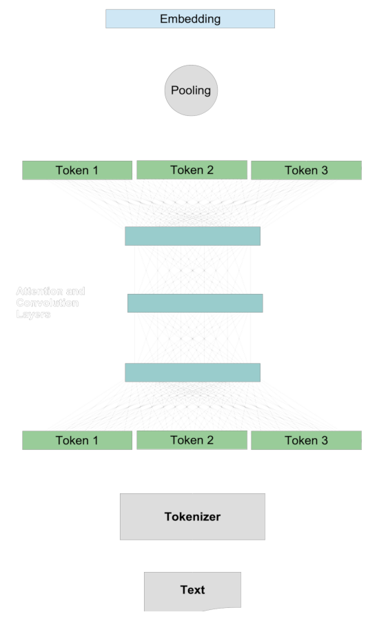
Then, when there is an embedding for each text, we compare them to each other, typically using the cosine metric or Hamming distance.
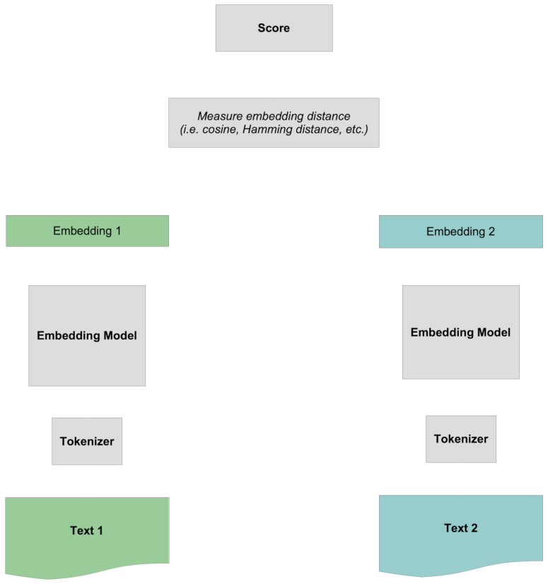
Scoring happens by comparing the two whole embeddings to each other, without any specific information about the tokens. All the interaction between tokens is “early” since it occurs before the two texts are compared to each other.
Reranking Models
Reranking models work differently.
First, instead of creating an embedding for any text, it takes one text, called a query, and a collection of other texts that we'll all target documents and then scores each target document with respect to the query text. These numbers are not normalized and are not like comparing embeddings, but they are sortable. The target documents that score the highest with respect to the query are the texts that are most semantically related to the query according to the model.
Let’s look at how this works concretely with the jina-colbert-v1-en reranker model, using the Jina Reranker API and Python.
The code below is also in a notebook which you can download or run in Google Colab.
You should install the most recent version of the requests library into your Python environment first. You can do so with the following command:
pip install requests -U
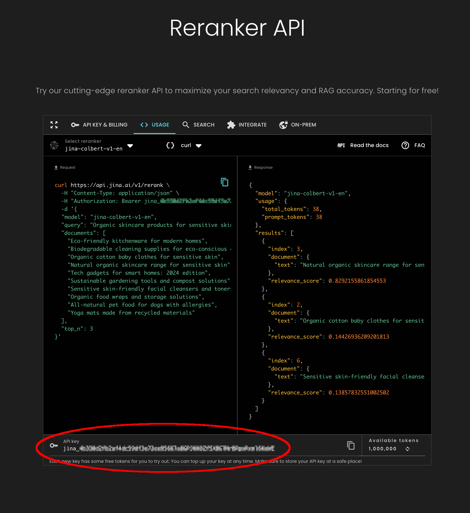
Next, visit the Jina Reranker API page and get a free API token, good for up to one million tokens of text processing. Copy the API token key from the bottom of the page, as shown below:
We’ll use the following query text:
- “Elephants eat 150 kg of food per day.”
And compare this query to three texts:
- “Elephants eat 150 kg of food per day.”
- “Every day, the average elephant consumes roughly 150 kg of plants.”
- “The rain in Spain falls mainly on the plain.”
The first document is identical to the query, the second is a rephrasing of the first, and the last text is completely unrelated.
Use the following Python code to get the scores, assigning your Jina Reranker API token to the variable jina_api_key:
import requests

url = "<https://api.jina.ai/v1/rerank>"
jina_api_key = "<YOUR JINA RERANKER API TOKEN HERE>"

headers = {
    "Content-Type": "application/json",
    "Authorization": f"Bearer {jina_api_key}"
}
data = {
    "model": "jina-colbert-v1-en",
    "query": "Elephants eat 150 kg of food per day.",
    "documents": [
        "Elephants eat 150 kg of food per day.",
        "Every day, the average elephant consumes roughly 150 kg of food.",
        "The rain in Spain falls mainly on the plain.",
    ],
    "top_n": 3
}

response = requests.post(url, headers=headers, json=data)
for item in response.json()['results']:
    print(f"{item['relevance_score']} : {item['document']['text']}")
Running this code from a Python file or in a notebook should produce the following result:
11.15625 : Elephants eat 150 kg of food per day.
9.6328125 : Every day, the average elephant consumes roughly 150 kg of food.
1.568359375 : The rain in Spain falls mainly on the plain.
The exact match has the highest score, as we would expect, while the rephrasing has the second highest, and a completely unrelated text has a much lower score.
Scoring using ColBERT
What makes ColBERT reranking different from embedding-based scoring is that the tokens of the two texts are compared to each other during the scoring process. The two texts never have their own embeddings.
First, we use the same architecture as embedding models to create new representations for each token that include context information from the text. Then, we compare each token from the query with each token from the document.
For each token in the query, we identify the token in the document that has the strongest interaction with it, and sum over those interaction scores to calculate a final numerical value.
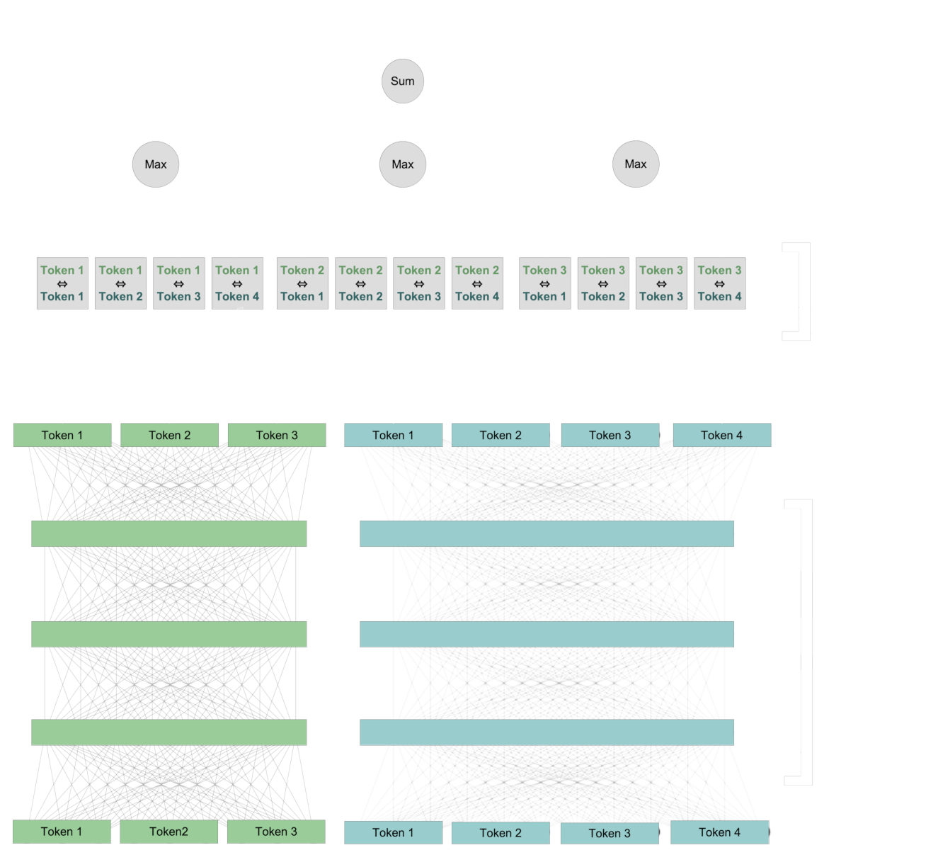
This interaction is “late”: Tokens interact across the two texts when we are comparing them to each other. But remember, the “late” interaction doesn’t exclude the “early” interaction. The token vectors pairs being compared already contain information about their specific contexts.
This late interaction scheme preserves token-level information, even if that information is context-specific. That enables us to see, in part, how the ColBERT model calculates its score because we can identify which pairs of contextualized tokens contribute to the final score.
Explaining Rankings with Heat Maps
Heat maps are a visualization technique that’s useful for seeing what’s going on in Jina-ColBERT when it creates scores. In this section, we’ll use the seaborn and matplotlib libraries to create heat maps from the late interaction layer of jina-colbert-v1-en, showing how the query tokens interact with each target text token.
Set-Up
We have created a Python library file containing the code for accessing the jina-colbert-v1-en model and using seaborn, matplotlib and Pillow to create heatmaps. You can download this library directly from GitHub, or use the provided notebook on your own system, or on Google Colab.
First, install the requirements. You will need the latest version of the requests library into your Python environment. So, if you have not already done so, run:
pip install requests -U
Then, install the core libraries:
pip install matplotlib seaborn torch Pillow
Next, download jina_colbert_heatmaps.py from GitHub. You can do that via a web browser or at the command line if wget is installed:
wget https://raw.githubusercontent.com/jina-ai/workshops/main/notebooks/heatmaps/jina_colbert_heatmaps.py
With the libraries in place, we need to only declare one function for the rest of this article:
from jina_colbert_heatmaps import JinaColbertHeatmapMaker

def create_heatmap(query, document, figsize=None):
    heat_map_maker = JinaColbertHeatmapMaker(jina_api_key=jina_api_key)
    # get token embeddings for the query
    query_emb = heat_map_maker.embed(query, is_query=True)
    # get token embeddings for the target document
    document_emb = heat_map_maker.embed(document, is_query=False)
    return heat_map_maker.compute_heatmap(document_emb[0], query_emb[0], figsize)
Results
Now that we can create heat maps, let’s make a few and see what they tell us.
Run the following command in Python:
create_heatmap("Elephants eat 150 kg of food per day.", "Elephants eat 150 kg of food per day.")The result will be a heat map that looks like this:
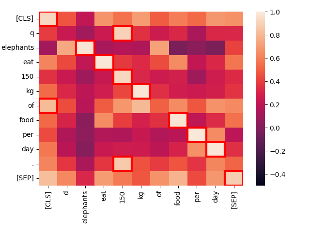
This is a heat map of the activation levels between pairs of tokens when we compare two identical texts. Each square shows the interaction between two tokens, one from each text. The extra tokens [CLS] and [SEP] indicate the beginning and the end of the text respectively, and q and d are inserted right after the [CLS] token in queries and target documents respectively. This allows the model to take into account interactions between tokens and the beginning and ends of texts but also allows token representations to be sensitive to whether they are in queries or targets.
The brighter the square, the more interaction there is between the two tokens, which is indicative of being semantically related. Each token pair’s interaction score is in the range -1.0 to 1.0. The squares highlighted by a red frame are the ones that count towards the final score: For each token in the query, it’s highest interaction level with any document token is the value that counts.
The best matches — the brightest spots — and the red-framed maximum values are almost all exactly on the diagonal, and they have very strong interaction. The only exceptions are the “technical” tokens [CLS], q, and d, as well as the word “of” which is a high-frequency “stop word” in English that carries very little independent information.
Let’s take a structurally similar sentence — “Cats eat 50 g of food per day.” — and see how the tokens in it interact:
create_heatmap("Elephants eat 150 kg of food per day.", "Cats eat 50 g of food per day.")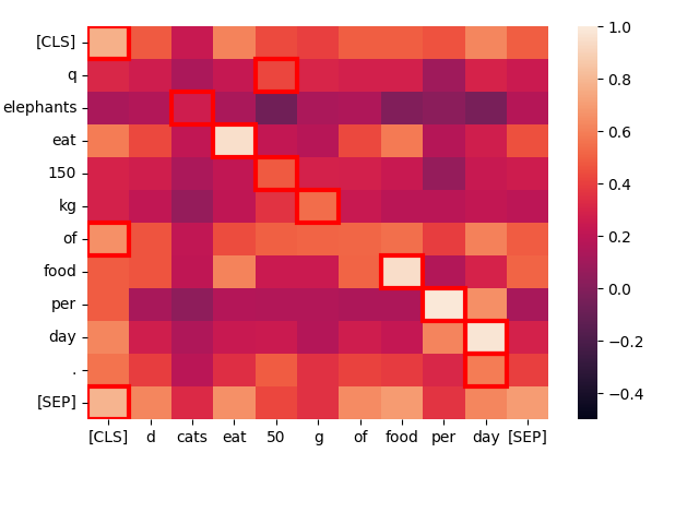
Once again, the best matches are primarily on the diagonal because the words are frequently the same and the sentence structure is nearly identical. Even “cats” and “elephants” match, because of their common contexts, although not very well.
The less similar the context, the worse the match. Consider the text “Employees eat at the company canteen.”
create_heatmap("Elephants eat 150 kg of food per day.", "Employees eat at the company canteen.")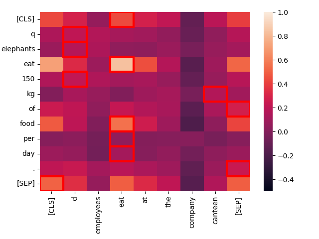
Although structurally similar, the only strong match here is between the two instances of “eat.” Topically, these are very different sentences, even if their structure are highly parallel.
Looking at the darkness of the colors in the red-framed squares, we can see how the model would rank them as matches for “Elephants eat 150 kg of food per day”, and jina-colbert-v1-en confirms this intuition:
| Score | Text |
|---|---|
| 11.15625 | Elephants eat 150 kg of food per day. |
| 8.3671875 | Cats eat 50 g of food per day. |
| 3.734375 | Employees eat at the company canteen. |
Now, let’s compare “Elephants eat 150 kg of food per day.” to a sentence that has essentially the same meaning but a different formulation: “Every day, the average elephant consumes roughly 150 kg of food.”
create_heatmap("Elephants eat 150 kg of food per day.", "Every day, the average elephant consumes roughly 150 kg of food.")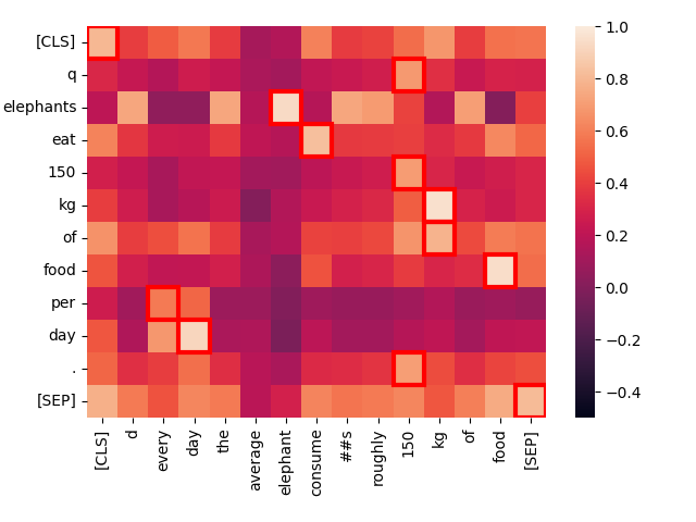
Notice the strong interaction between “eat” in the first sentence and “consume” in the second. The difference in vocabulary doesn’t prevent Jina-ColBERT from recognizing the common meaning.
Also, “every day” strongly matches “per day”, even though they are in completely different places. Only the low-value word “of” is an anomalous non-match.
Now, let’s compare the same query with a totally unrelated text: “The rain in Spain falls mainly on the plain.”
create_heatmap("Elephants eat 150 kg of food per day.", "The rain in Spain falls mainly on the plain.")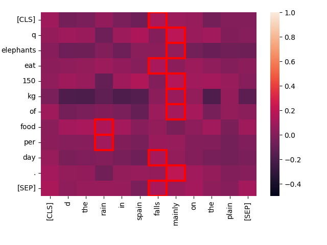
You can see that “best match” interactions score much lower for this pair, and there is very little interaction between any of the words in the two texts. Intuitively, we would expect it to score poorly compared to “Every day, the average elephant consumes roughly 150 kg of food”, andjina-colbert-v1-en agrees:
| Score | Text |
|---|---|
| 9.6328125 | Every day, the average elephant consumes roughly 150 kg of food. |
| 1.568359375 | The rain in Spain falls mainly on the plain. |
Long Texts
These are toy examples to demonstrate the workings of ColBERT-style reranker models. In information retrieval contexts, like retrieval-augmented generation, queries tend to be short texts while matching candidate documents tend to be longer, often as long as the input context window of the model.
Jina-ColBERT models all support 8192 token input contexts, equivalent to roughly 16 standard pages of single-spaced text.
We can generate heat maps for these asymmetric cases too. For example, let’s take the first section of the Wikipedia page on Indian Elephants:
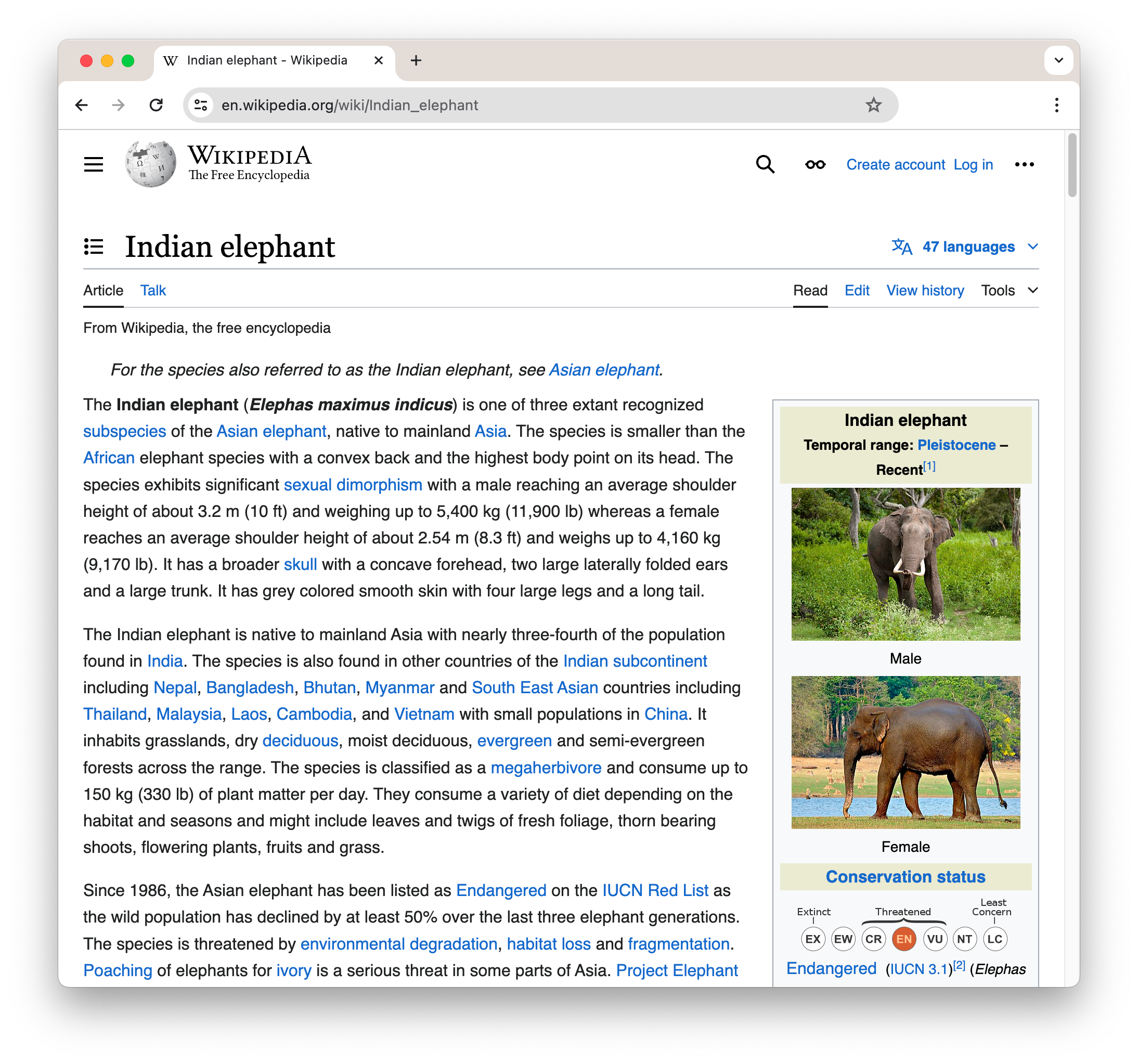
To see this as plain text, as passed to jina-colbert-v1-en, click this link.
This text is 364 words long, so our heat map won’t look very square:
create_heatmap("Elephants eat 150 kg of food per day.", wikipedia_elephants, figsize=(50,7))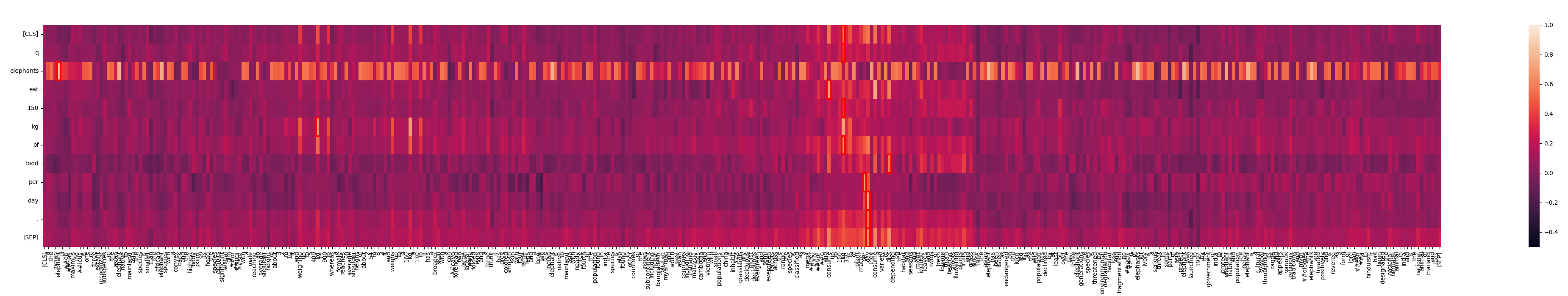
We see that “elephants” matches a lot of places in the text. This isn’t surprising in a text about elephants. But we can also see one area where there is a lot stronger interaction:
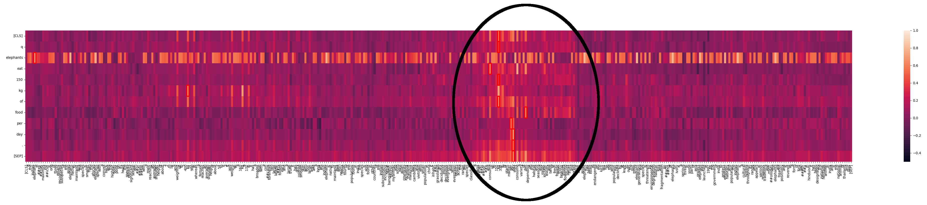
What’s going on here? With Jina-ColBERT, we can find the part of the longer text that this corresponds to. It turns out it’s the fourth sentence of the second paragraph:
The species is classified as a megaherbivore and consume up to 150 kg (330 lb) of plant matter per day.
This restates the same information as in the query text. If we look at the heat map for just this sentence we can see the strong matches:
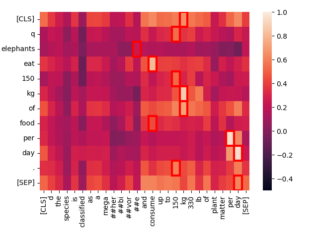
Jina-ColBERT provides you with the means to see exactly what areas in a long text caused it to match the query. This leads to better debugging, but also to greater explainability. It doesn’t take any sophistication to see how a match is made.
Explaining AI outcomes with Jina-ColBERT
Embeddings are a core technology in modern AI. Almost everything we do is based on the idea that complex, learnable relationships in input data can be expressed in the geometry of high-dimensional spaces. However, it’s very difficult for mere humans to make sense of spatial relationships in thousands to millions of dimensions.
ColBERT is a step back from that level of abstraction. It’s not a complete answer to the problem of explaining what an AI model does, but it points us directly at which parts of our data are responsible for our results.
Sometimes, AI has to be a black box. The giant matrices that do all the heavy lifting are too big for any human to keep in their heads. But the ColBERT architecture shines a little bit of light into the box and demonstrates that more is possible.
The Jina-ColBERT model is currently available only for English (jina-colbert-v1-en) but more languages and usage contexts are on their way. This line of models, which not only perform state-of-the-art information retrieval but can tell you why they matched something, demonstrates Jina AI's commitment to making AI technologies both accessible and useful.