Benchmark Vector Search Databases with One Million Data

In DocArray, Documents inside a DocumentArray can live in a document store instead of in memory. The benefit of using an external store over an in-memory store is often about longer persistence and faster retrieval.

Document Store

Documents inside a DocumentArray can live in a document store instead of in memory, e.g. in SQLite, Redis. The benefit of using an external store over an in-memory store is often about longer persistence and faster retrieval. The look-and-feel of a DocumentArray with external store is almost the ...

DocArray 0.18.2 Documentation

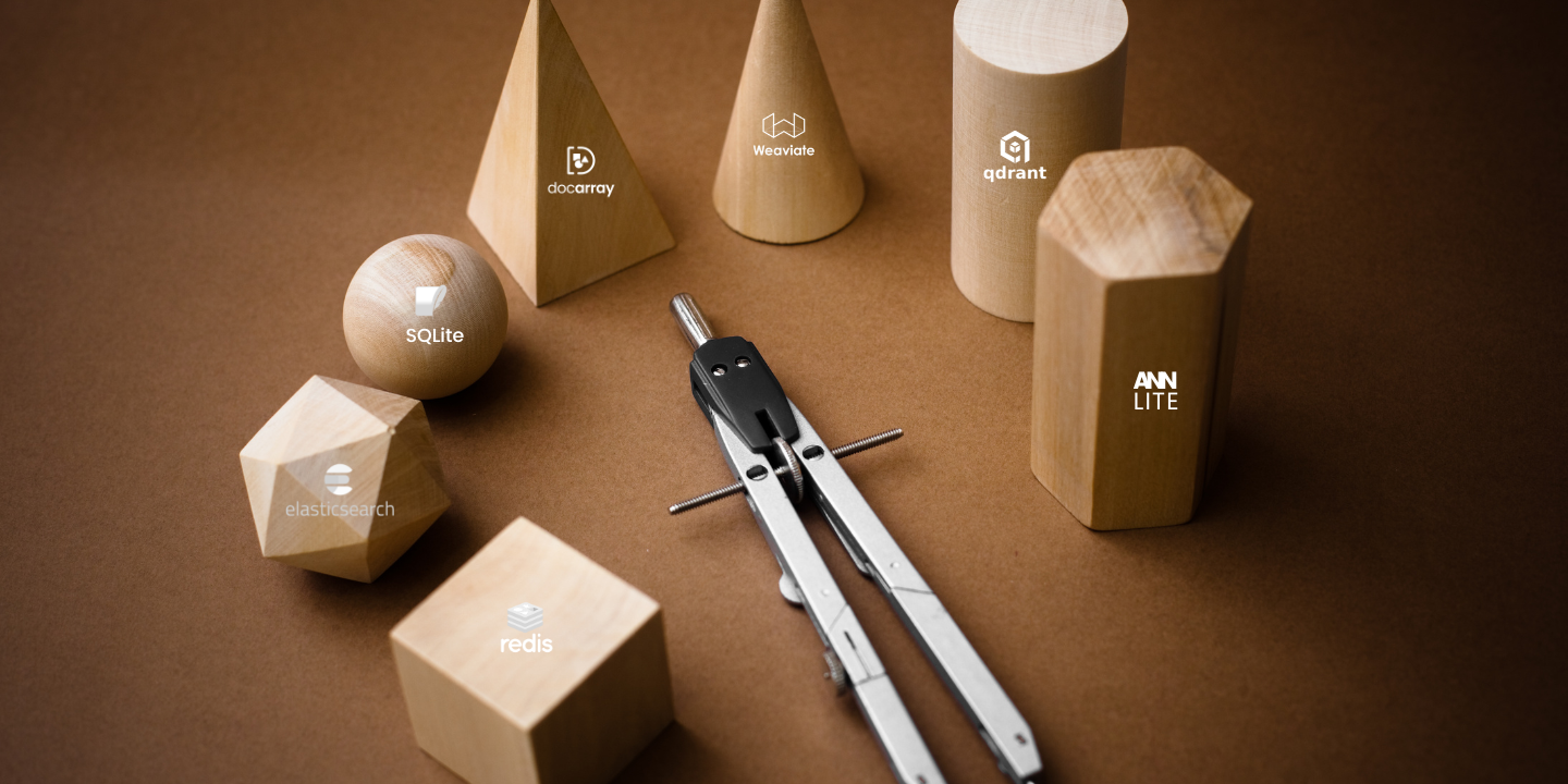
Today, DocArray supports six external stores including SQLite, Weaviate, Qdrant, Elasticsearch, Redis and AnnLite. Apart from SQLite, all other backends support approximate nearest neighbour search. The look-and-feel of a DocumentArray with an external store is almost the same as a regular in-memory DocumentArray. This lets you easily switch between backends under the same DocArray idiom. For example, to use Elasticsearch as the backend, simply:

from docarray import DocumentArray

da = DocumentArray(storage='elasticsearch', config={'n_dim': 128})

Or if you want to use Qdrant, you can just change one parameter:

from docarray import DocumentArray

da = DocumentArray(storage='qdrant', config={'n_dim': 128})

You get the idea!

Ever wonder about which document store is best for your use case? Here's a comprehensive benchmark to help guide you.

Methodology

We created a DocumentArray with one million Documents based on sift1m, a dataset containing 1 million objects (each of 128 dimensions) and using L2 distance metrics.

sift1m | TensorFlow Datasets

Pre-trained embeddings for approximate nearest neighbor search using theEuclidean distance. This dataset consists of two splits: 1. ‘database’: consists of 1,000,000 data points, each has features: ‘embedding’ (128 floats), ‘index’ (int64), ‘neighbors’ (empty list). 2. ‘test’: consists of…

TensorFlow

We benchmarked the document stores as summarized below:

Core tasks

We focused on the following tasks on every document store:

1. Create: Add one million Documents to the document store via extend() and backend capabilities when applicable.
2. Read: Retrieve existing Documents from the document store by .id, i.e. da['some_id'].
3. Update: Update existing Documents in the document store by .id, i.e. da['some_id'] = Document(...).
4. Delete: Delete Documents from the document store by .id, i.e. del da['some_id']
5. Find by condition: Search existing Documents by .tags via find() in the document store by boolean filters and use backend side filtering when possible, as described in Query by Conditions.
6. Find by vector: Retrieve existing Documents by .embedding via find() using nearest neighbor search or approximate nearest neighbor search, as described in Find Nearest Neighbours.

The above tasks are often atomic operations in the high-level DocArray API. Hence, understanding their performance gives users a good estimation of the experience when using DocumentArray with different backends.

Parametric combinations

Most of these document stores use their own implementation of HNSW (an approximate nearest neighbor search algorithm) but with different parameters:

• ef_construct - the HNSW build parameter that controls the index time/index accuracy. Higher ef_construct leads to longer construction, but better index quality.
• m - maximum connections, the number of bi-directional links created for every new element during construction. Higher m works better on datasets with high intrinsic dimensionality and/or high recall, while lower m works better for datasets with low intrinsic dimensionality and/or low recall.
• ef - the size of the dynamic list for the nearest neighbors. Higher ef at search leads to more accuracy but slower performance.

Experiment setup

We are interested in the single query performance on the above six tasks with different combinations of the above three parameters. Single query performance is measured by evaluating one Document at a time, repeatedly for tasks 2, 3, 4, 5, and 6. Finally the average number is reported.

We now elaborate the setup of our experiments. First some high-level statistics of the experiment:

Each Document follows the structure:

{
  "id": "94ee6627ee7f582e5e28124e78c3d2f9",
  "tags": {"i": 10},
  "embedding": [0.49841760378680844, 0.703959752118305, 0.6920759535687985, 0.10248648858410625, ...]
}

We use Recall@K value as an indicator of search quality. The in-memory and SQLite store do not implement approximate nearest neighbor search but use exhaustive search instead. Hence, they give the maximum Recall@K but are the slowest.

The experiments were conducted on an AWS EC2 t2.2xlarge instance (Intel Xeon CPU E5-2676 v3 @ 2.40GHz) with Python 3.10.6 and DocArray 0.18.2.

As Weaviate, Qdrant, Elasticsearch, and Redis follow a client/server pattern, we set them up with their official Docker images in a single node configuration, with 32 GB of RAM allocated. That is, only 1 replica and shard are operated during the benchmarking. We did not opt for a cluster setup because our benchmarks mainly aim to assess the capabilities of a single instance of the server.

docarray/benchmarking_sift1m.py at main · docarray/docarray

🧬 The data structure for unstructured multimodal data · Neural Search · Vector Search · Document Store - docarray/benchmarking_sift1m.py at main · docarray/docarray

GitHubdocarray

Latency result

In-Memory

SQLite

AnnLite

Qdrant

Weaviate

Elasticsearch

Redis

QPS result

When we consider each Document as a query, we can convert the above metrics into queries per second (QPS). Higher values are better.

In-memory

SQLite

AnnLite

Qdrant

Weaviate

Elasticsearch

Redis

Vector search recall & QPS

In particular to the find by vector queries task, the chart below depicts Recall@10 (the fraction of true nearest neighbors found, on average over all queries) against the QPS. The smaller the time values and the more upper-right in the chart, the better.

Rationale on experiment design

Our experiments are designed to be fair and the same across all backends while favouring document stores that benefit DocArray users the most. Note that such a benchmark was impossible to set up before DocArray, as each store has its own API and the definition of a task varies.

Our benchmark is based on the following principles:

• Cover the most important operations: We understand that some backends are better at some operations than others, and some offer better quality. Therefore, we try to benchmark on six operations (CRUD + Find by vector + Find by condition) and report quality measurement (Recall@K).
• Not just speed, but also quality: We show the trade-off between quality and speed as you tune your parameters in each document store.
• Same experiment, same API: DocArray offers the same API across all backends and therefore we built on top of it the same benchmarking experiment. Furthermore, we made sure to run the experiment with a series of HNSW parameters for backends that support approximate nearest neighbor search. All backends are run on official Docker containers, local to the DocArray client which allows having similar network overhead. We also allocate the same resources for those Docker containers and all servers are run in a single node setup.
• Benefit users as much as possible: We offer the same conditions and resources to all backends, but our experiment favors backends that use resources efficiently. Therefore, some backends might not use the network, or use gRPC instead of HTTP, or use batch operations. We’re okay with that, as long as it benefits the DocArray and Jina user.
• Open to improvements: We are constantly improving the performance of storage backends from the DocArray side and updating benchmarks accordingly. If you believe we missed an optimization (e.g. perform an operation in batches, benefit from a recent feature in upstream, avoid unnecessary steps), feel free to raise a PR or issue. We’re open to your contributions!

Known limitations

• Incompleteness on the document stores: We do not benchmark algorithms or ANN libraries like Faiss, Annoy, ScaNN. We only benchmark backends that can be used as document stores. In fact, we do not benchmark HNSW itself, but it is used by some backends internally. Other storage backends that support vector search are not yet integrated with DocArray. We’re open to contributions to DocArray’s repository to support them.
• Client/server setup introduces random network latency: Although a real-life scenario would be the clients and server living on different machines with potentially multiple clients in parallel, we chose to keep both on the same machine and have only one client process to minimize network overhead.
• Benchmarks are conducted end-to-end: We benchmark function calls from DocArray, not just the underlying backend vector database. Therefore, results for a particular backend can be influenced (positively or negatively) by our interface. If you spot bottlenecks we would be thrilled to know about them and improve our code accordingly.
• We use similar underlying search algorithms but different implementations: In this benchmark we try a set of parameters ef, ef_construct and max_connections from HNSW applied equally on all backends. Note that there might be other parameters that storage backends can fix than might or might not be accessible and can have a big impact on performance. This means that even similar configurations cannot be easily compared.
• Benchmark is for DocArray users, not for research: This benchmark showcases what a user can expect to get from DocArray without tuning hyper-parameters of a vector database. In practice, we strongly recommend tuning them to achieve high quality results.

Conclusions

We hope our benchmark result can help users select the store that suits their use cases. Depending on the dataset size and the desired quality, some stores may be preferable than others. Here are some of our conclusions:

• If your dataset has fewer than 10,000 Documents, you should just use the in-memory DocumentArray as-is to enjoy the best quality for nearest neighbor search with reasonable latency (e.g. ~20 ms/query).
• If your dataset is large but still fits into memory (say 1 million Documents), Redis and AnnLite offer great speed in CRUD and vector search operations. In particular, AnnLite is designed as a monolithic package, which saves a lot network overhead unlike other backends. Unfortunately, this also means one can not scale-out AnnLite natively. Nonetheless, if you are using DocArray with Jina together, you can always leverage Jina’s sharding features, an agnostic solution to scale out any document store. This of course also includes AnnLite.

Scale out with replicas and shards

A Jina Flow orchestrates multiple Executor s. By default, an Executor runs with a single replica and shard. Some Executors in the Flow may be less performant than others, which could cause performance bottlenecks in an application. To solve this, you can configure the number of replicas and shard...

Jina 3.11.1 Documentation

• Finally, if your dataset does not fit in memory, and you do not care much about the speed of nearest neighbor search, you can use SQLite as storage. Otherwise, Weaviate, Qdrant and Elasticsearch are good options.