Embeddings in Depth

This article is the second in our series on embedding technology. In the previous article, we discussed embeddings in very abstract terms, but this one will be much more concrete. It explains where embeddings come from and how they are used.

An embedding is a mapping of objects to vectors. Those objects may be real things or digital objects like images and files.

For example, imagine a robot that harvests tomatoes:

This robot selects tomatoes on the vine that are ready to harvest, and then snips their stalks and takes them away. Recognizing which tomatoes are ripe is a good application of image embeddings. Each tomato on the vine is assigned a representative vector based on digital images taken by the robot’s cameras. It then uses these embeddings to decide whether or not to harvest a particular tomato.

Similarly, we might use embeddings to study and predict customer behavior. These embedding vectors stand in for a person — a real human being who presumably exists somewhere — but we construct their embedding vectors from digital information about that person. For a study of consumer buying behavior, this is likely to be some combination of demographic information and purchasing records.

In the previous article, we discussed how vectors are just ordered lists of numbers that we decide to interpret as points in a high-dimensional space. Data stored in a computer is also just an ordered list of numbers. Embeddings are, therefore, made by translating input vectors in one vector space — the one that contains the source data — into vectors in a different space called the embedding space.

But not just any mapping between vector spaces is an embedding. The translation into embeddings is purposeful. The placement of embedding vectors relative to each other should be informative in some way about the objects they represent.

Cosines: How We Compare Embeddings

When we use embeddings in applications, the thing we most often do is compare two embeddings and calculate how close or far apart they are. This is indicative of the similarity or dissimilarity of the objects those embeddings stand in for with respect to some set of properties.

To do this, we use a metric called the cosine. This section explains cosines and how we calculate them in high-dimensional vector spaces.

An embedding is a vector, and as we showed in the previous section, we can interpret a vector as a point in a multi-dimensional space. However, it also has an interpretation as a direction and magnitude. Traditionally, we visualize this interpretation with an arrow:

The direction of this three-dimensional vector is specified by the $(x,y,z)$ coordinates, and the magnitude is just the length of the vector, i.e., the distance from the coordinate $(x,y,z)$ to the origin at $(0,0,0)$. The length is calculated using a multidimensional extension of Pythagoras' theorem:

The double bars around a vector $\|\vec{v}\|$ indicate the vector's length (or magnitude).

We can see that different vectors can have the same direction but different lengths. For example, if we have the vectors $(4,2)$ and $(2,1)$, they have different lengths ($\sqrt{20} \approx 4.47$ and $\sqrt{5} \approx 2.23$ respectively) but they point in the same direction.

How do we know they point in the same direction? We measure the angle between the two vectors. If the angle is zero, they point in the same direction.

To show how this works, let’s consider two vectors: $\vec{a}=(3,2,5)$ and $\vec{b}=(4,5,2)$:

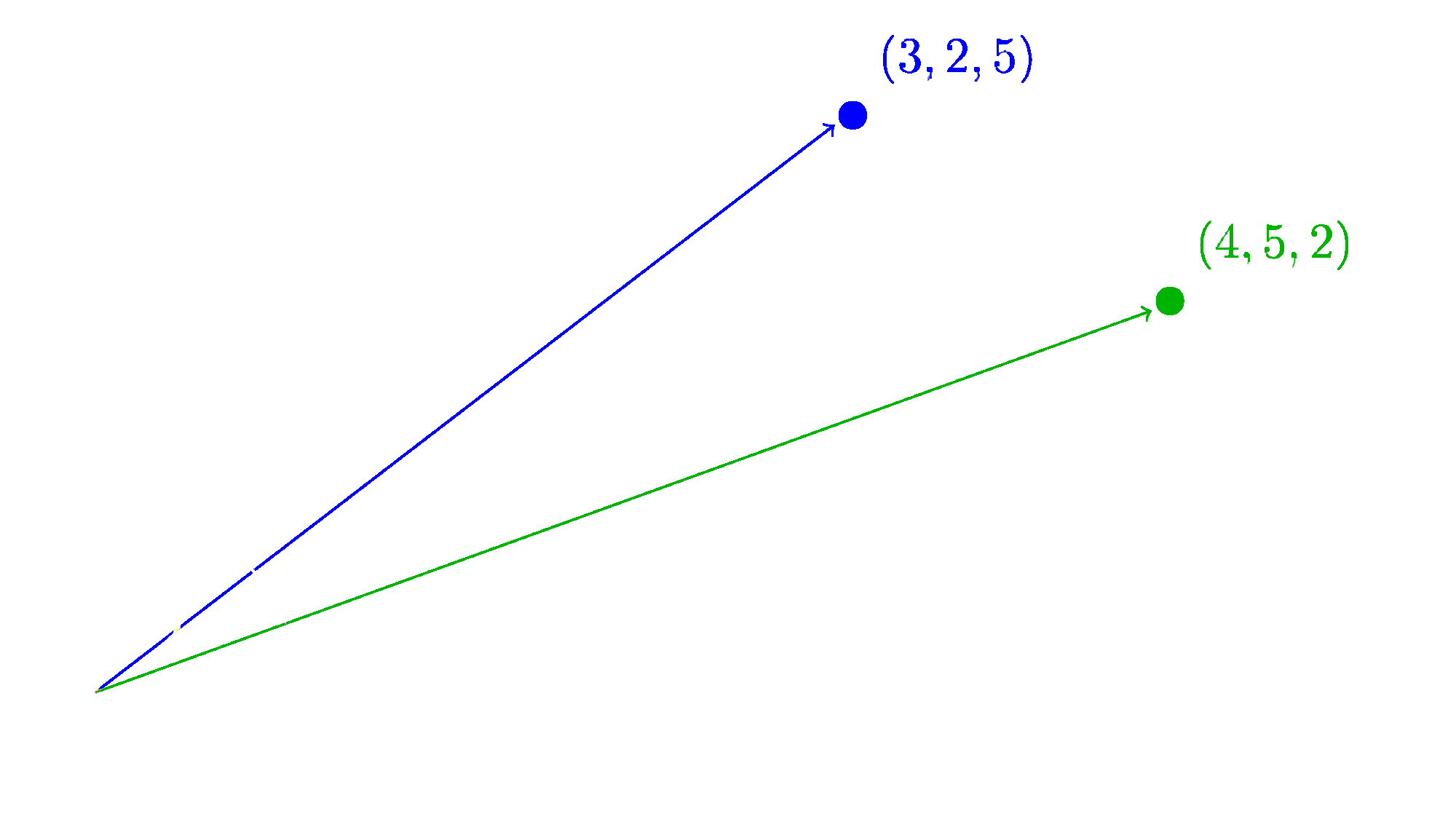
To calculate the angle, we have a formula that scales up to any number of dimensions: The cosine.

The cosine of the angle $\theta$ between vectors $\vec{a}$ and $\vec{b}$ is:

The numerator of this fraction, $a⋅b$, is the dot product of the two vectors, and it’s easy to calculate:

As for ‖a‖ and ‖b‖, those are the lengths of the two vectors: $\|\vec{a}\| = \sqrt{38} \approx 6.164$ and $\vec{b} = \sqrt{45} \approx 6.708$. Therefore, to calculate $cosθ$:

This cosine corresponds to an angle of approximately 39.3 degrees, but in machine learning, we typically stop once we’ve calculated the cosine because if all the numbers in both vectors are greater than zero, then the cosine of the angle will be between 0 and 1. A cosine of 1 means the angle between two vectors is 0 degrees, i.e., the vectors have the same direction (although they may have different lengths). A cosine of 0 means they have an angle of 90 degrees. i.e., they are perpendicular or orthogonal.

So let’s compare $\vec{a}=(4,2)$ and $\vec{b}=(2,1)$:

When the cosine of two vectors is one, they point in the same direction, even though they may have different lengths.

Another way to do the same operation is to take each vector and normalize it. Normalizing a vector means creating a new vector that points in the same direction but has a length of exactly 1. If two vectors point in the same direction, they will normalize to identical vectors.

To normalize a vector, divide it in each dimension by the vector’s length. If $\vec{v} = (3,2,5)$ and $\hat{v} = norm(\vec{v})$ then:

If two vectors $\vec{a}$ and $\vec{b}$ have an angle between them $\theta$, then their normalized forms $\hat{a}$ and $\hat{b}$ will have the same angle $\theta$ between them. Cosine is a measure that is indifferent to the magnitudes of vectors.

The reason for this is that the magnitudes of embedding vectors are not usually informative about anything. Most neural network architectures perform normalizations between some or all of their layers, rendering the magnitudes of embedding vectors typically useless.

Neural Networks As Vector Mappings

Embedding vectors work because they are placed so that things that have common properties have cosines that are closer to 1, and those that do not have cosines closer to 0. An embedding model takes input vectors and translates them into embedding vectors.

Although there are many techniques for performing such translations, today, embedding models are exclusively neural networks.

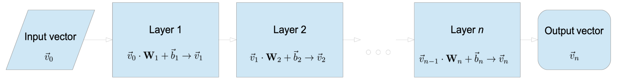
A neural network is a sequence of vector transformations. In formal mathematical terms, for each layer of the network, we multiply the vector output of the previous layer by a matrix, and then generally add a bias. A bias is a set of values that we add or subtract from the resulting vector. We take the result and make that the input to the next layer of the network.

More formally, the values of the $m$th layer of the network are $\vec{m}$ and are transformed into the values of the $n$th layer ($\vec{n}$) by:

Where $\textbf{W}$ is a matrix and $\vec{bias}$ is the vector of bias values.

It’s customary to think of it as a network of “nodes” bearing numerical values, connected by “weights”. This is truer to the roots of neural network theory but is exactly equivalent to multiplying a vector by a matrix.

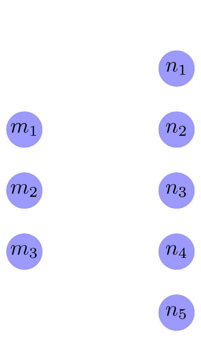
If we have a vector $\vec{m} = (m_1,m_2m_3)$, this one neural network layer transforms it into a vector $\vec{n} = (n_1,n_2,n_3,n_4,n_5)$. It does that by multiplying the values in $\vec{m}$ by a set of weights (also called parameters), then adding them up, and adding the bias vector $\vec{bias} = (bias_1,bias_2,bias_3,bias_4,bias_5)$

Each line between nodes in the diagram above is one weight. If we designate the weight from $m_1$ to $n_1$ as $w_{11}$, from $m_2$ to $n_3$ as $w_{23}$, etc., then:

In matrix algebra notation, this is the same as multiplying the 3-dimensional vector $\vec{n}$ by a $3x5$ matrix to get $\vec{m}$:

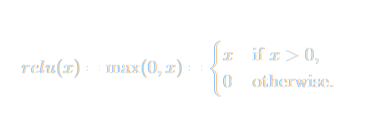
Neural networks have multiple layers, so the output of this matrix multiplication is multiplied by another matrix and then another, typically with some kind of thresholding or normalization between multiplications and sometimes other tricks. The most common way of doing this today is to apply the ReLU (rectified linear activation unit) activation function. If the value of any node is below zero, it’s replaced with a zero, and otherwise, left unchanged.

Otherwise, a neural network is just a series of transformations like the one above from $\vec{m}$ to $\vec{n}$.

This structure has some important properties. The most important is that:

It may be impractical to construct a large enough network for a given problem, and there may be no procedure for correctly calculating the weights. AI models are not guaranteed in advance to be able to learn or perform any task at all.

What happens in practice is that neural networks approximate a solution by learning from examples. How good a solution that approximation is depends on a lot of factors and can’t typically be known in advance of training a model.

There is an aphorism attributed to the British statistician George Box:

Neural networks can be very good approximations, but they are still approximations, and it’s not possible to know for certain how good they are at something until you put them into production. The real measure of an AI model is its usefulness, and that’s hard to know in advance.

Turning Problems Into Vector Mappings

Defining neural networks as mappings from one vector space to another sounds very limiting. We don’t naturally see the kinds of things we want AI models to do in those terms.

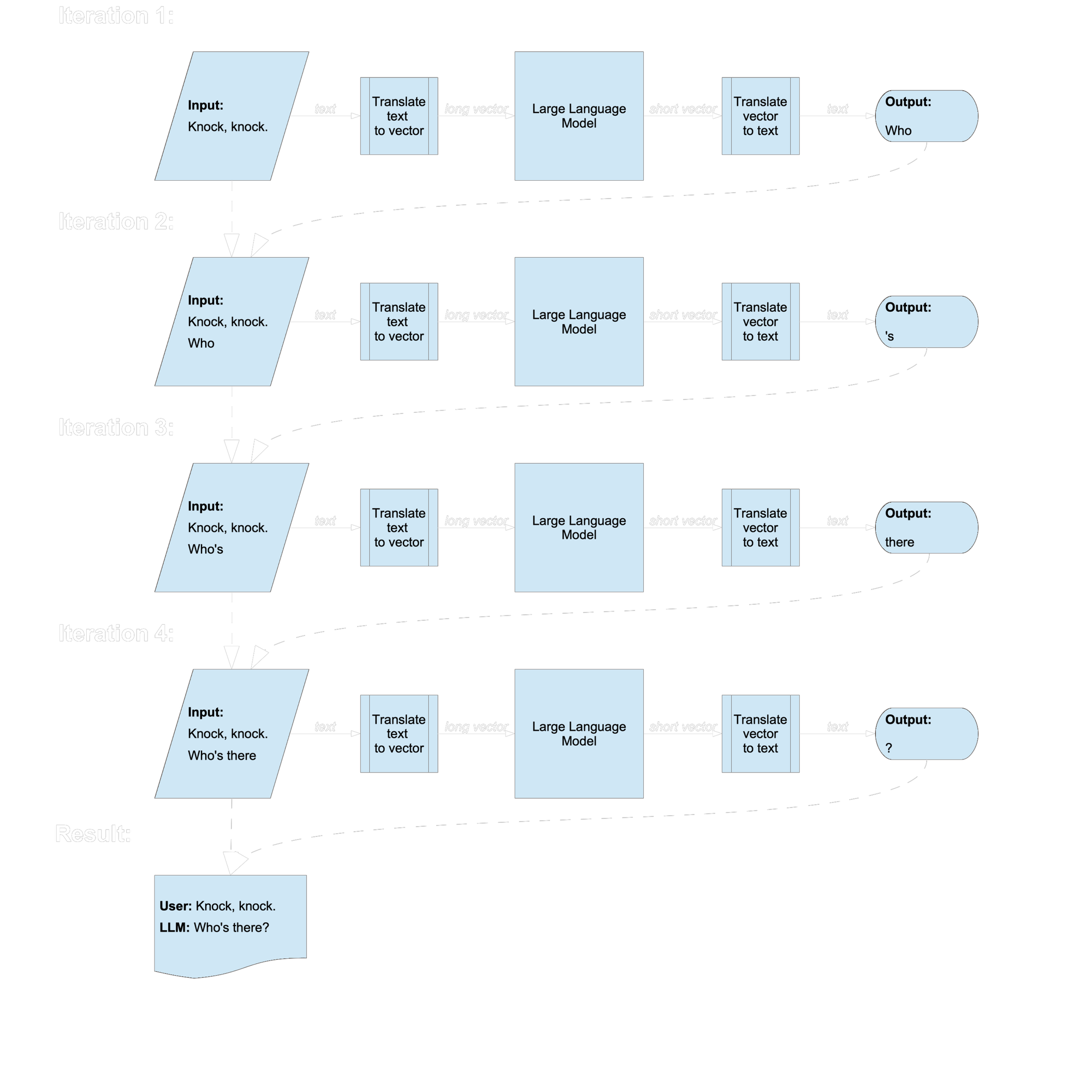
However, many of the most visible developments in recent AI are really just ways of using vector-to-vector mappings in clever ways. Large language models like ChatGPT translate input texts, rendered as vectors, into vectors that designate a single word. They write texts by adding the single-word output to the end of the input and then running again to get the next word.

It may take some creativity and engineering to find a way to express some task as a vector mapping, but as recent developments show, it is surprisingly often possible.

Where Do Embeddings Fit In?

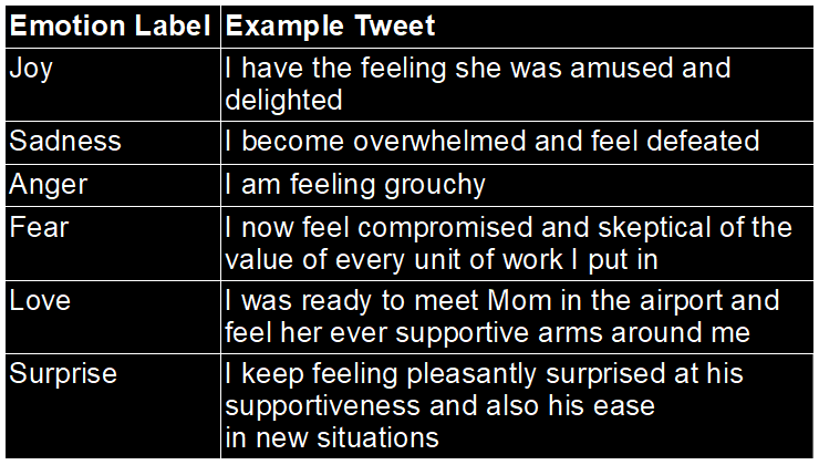
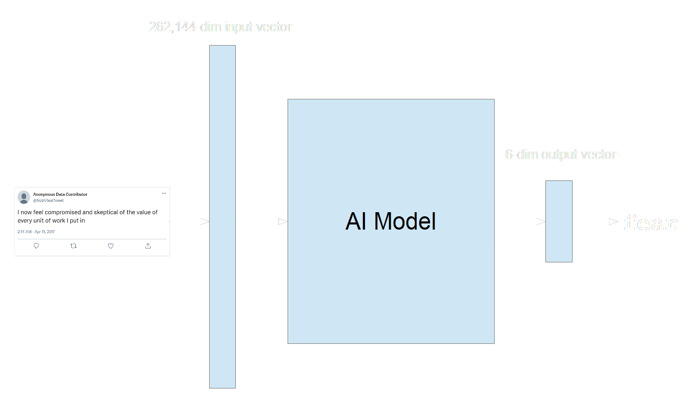
When you train an AI model, you do it with some goal in mind. In the typical scenario, you have training data that consists of inputs and matching correct outputs. For example, let’s say you want to classify tweets by their emotional content. This is a common benchmarking task used to evaluate text AI models.

One widely used dataset (DAIR.AI Emotion) sorts tweets into eight emotional categories:

To train a model to do this task, you need to decide two things:

1. How to map the output category labels to vectors.
2. How to map the input texts to vectors

The easiest way to encode these emotion labels is to create six-dimensional vectors where each value corresponds to one category. For example, if we make a list of emotions, like the one above, “anger” is the third in the list. So if a tweet has angry content, we train the network to output a six-dimensional vector with zero values everywhere except the third item in it, which is set to one:

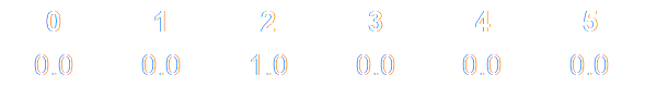
This approach is called zero-hot encoding among AI engineers.

We also have to encode the tweets as vectors. There is more than one way to do this, but most text-processing models follow broadly the same pattern:

First, input texts are split into tokens, which you can understand as something like splitting it into words. The exact mechanisms vary somewhat, but the procedure broadly follows the following steps:

1. Normalize the case, i.e., make everything lowercase.
2. Split a text on punctuation and spaces.
3. Look up each resulting subsegment of text in a dictionary (which is a part of the AI model bundle) and accept it if it is in the dictionary.
4. For segments not in the dictionary, split them into the smallest number of parts that are in the dictionary, and then accept those segments.

So, for example, let’s say we wanted an embedding for this famous line from Alice in Wonderland:

Jina Embeddings’ text tokenizer will split it up into 18 tokens like this:

[CLS] why , sometimes i ' ve believed as many as six impossible 
things before breakfast . [SEP]

The [CLS] and [SEP] are special tokens added to the text to indicate the beginning and end, but otherwise, you can see that the splits are between words on spaces and between letters and punctuation.

If the tokenizer encounters a sentence with words that are not in the dictionary, it tries to match the parts to entries in its dictionary. For example:

This is rendered in the Jina tokenizer as:

[CLS] k ##la ##at ##u bar ##ada nik ##to [SEP]

The ## indicates a segment appearing elsewhere than the beginning of a word.

This approach guarantees that every possible string can be tokenized and can always be processed by the AI model, even if it’s a new word or a nonsense string of letters.

Once the input text is transformed into a list of tokens, we replace each token with a unique vector from a lookup table. Then, we concatenate those vectors into one long vector.

Many text-processing AI models (including Jina Embeddings 2 models) use vectors of 512 dimensions for each token. All text-processing models are limited in the number of tokens they can accept as input. Jina Embeddings 2 models accept 8,192 tokens, but most models only take 512 or fewer.

If we use 512 for this example, then to do emotion classification for these tweets, we need to build a model that takes an input vector of $512 \times 512 = 262144$ dimensions, and outputs a vector of 6 dimensions:

Neural networks are often presented as a kind of black box in which the parts on the inside are not described in depth. This is not wrong, but it’s not very informative. In practice, large, modern AI models tend to have three components, although this is not always true, and the boundaries between them are not always clear:

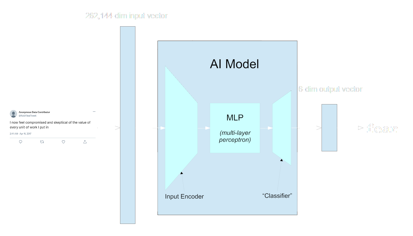
The vocabulary for some of this is not entirely codified, and this schema does not apply to all AI models, but in general, a trained model has three parts:

1. An input processor or encoder
   
   Especially for networks that take in very large input vectors, there is some part of the network devoted to correlating all parts of the input with each other. This section of the network can be very large, and it can be structurally complex. Many of the biggest breakthroughs in AI in the last two decades have involved innovative structures in this part of the model.
   
2. A multi-layer perceptron
   
   There isn’t a consistent term for this “middle” part of the model, but “MLP” or “multi-layer perceptron” appear to be the most common terms in the technical literature. The term itself is a bit old-fashioned, recalling the “perceptron”, a kind of small single-layer neural network invented in the 1950s that is ancestral to modern AI models.
   
   The MLP typically consists of a number of connected layers of the same size. For example, the smallest of the ViT image processing models has twelve layers with 192 dimensions in each, while the largest has 24 layers, each with 768 dimensions.
   
   The size and structure of the MLP are key design variables in an AI model.
   
3. The “Classifier”
   
   This is usually the smallest part of the model, typically much smaller than the MLP. It may be as small as one layer but typically has more in modern models. This part of the model translates the output of the MLP into the exact form specified for the output, like the thousand-dimension one-hot vectors used for Imagenet-1k. It may not actually be a classifier. This final section of the model may be trained to do some other task.

The size of the input encoder is mostly determined by your planned input sizes and the size of the first layer of the MLP. The size of the “classifier” is mostly determined by the training objective and the size of the last layer of the MLP. You have relatively few design choices in those areas. The MLP is the only part where you can make free decisions about your model.

The size of the MLP is a design choice balancing three factors:

• Smaller MLPs learn faster, run faster, and take less memory than large MLPs.
• Large MLPs typically learn more and perform better, all else being equal.
• Large MLPs are more likely to “overfit” than small MLPs. There is a risk that instead of generalizing from their training examples, they will memorize them and not learn effectively.

The optimal balance depends on your use case and context, and it is very difficult to calculate the optimum in advance.

Most of the learning takes place in the MLP. The MLP learns to recognize those features of the inputs that are useful in calculating the correct output. The last layer of the MLP outputs vectors that are closer together the more they share those features. The “classifier” then has the relatively easy task of translating that into the correct output, like what class a particular input belongs to..

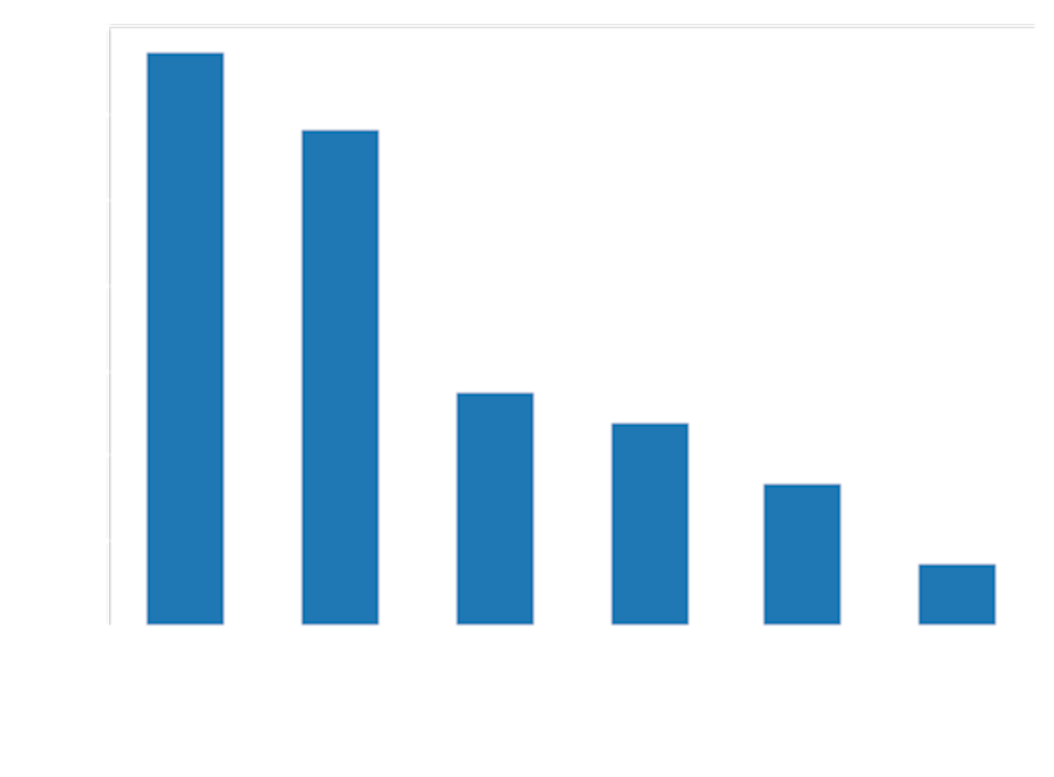
So, for example, if we train a text classifier with the six emotion labels from our dataset, we would expect the outputs of the MLP to be a high-dimensional analog of something like this:

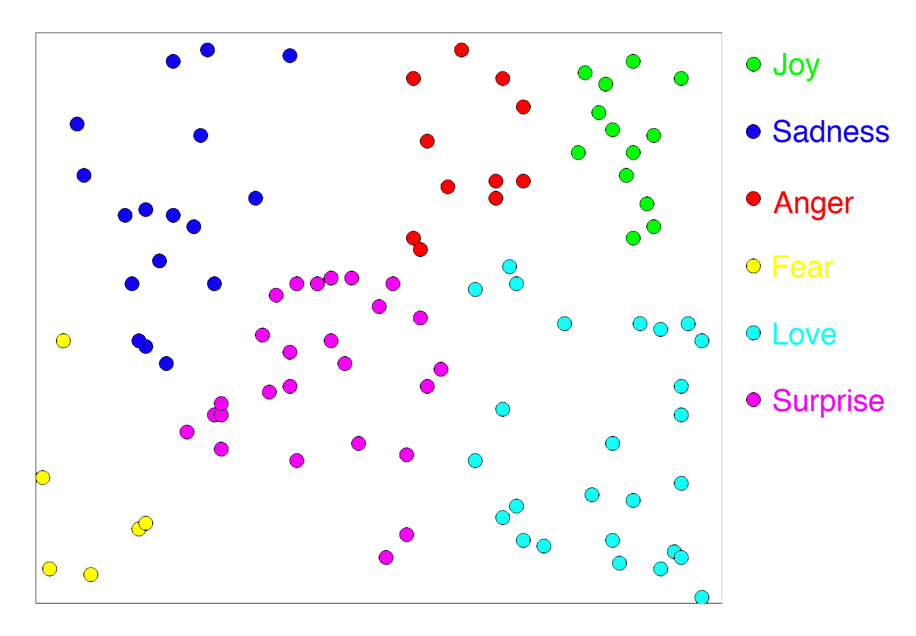
In short, the output of the last layer of the MLP has all the properties we want in an embedding: It puts similar things close together and dissimilar things further apart.

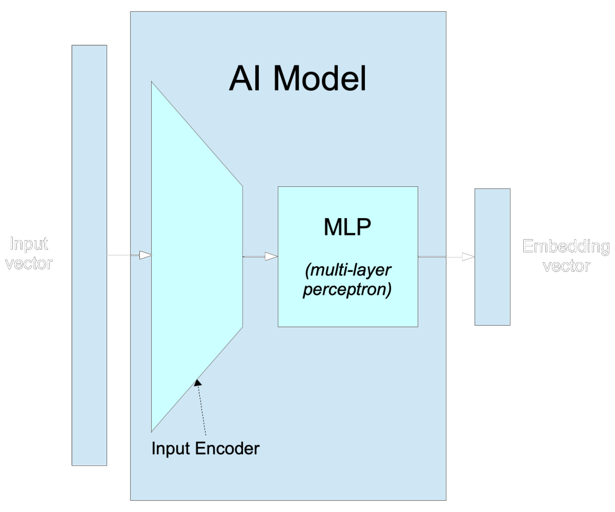
We typically construct embedding models by taking a model we’ve trained for something — often classification, but not necessarily — and throwing away the “classifier” part of the model. We just stop at the last layer of the MLP and use its outputs as embeddings.

There are four key points to take from this:

1. Embeddings put things close to each other that are similar based on a set of features.
2. The set of features that embeddings encode is not usually specified in advance. It comes from training a neural network to do a task and consists of the features the model discovered were relevant to doing that task.
3. Embedding vectors are typically very high-dimensional but are usually much, much smaller than input vectors.
4. Most models have an embedding layer in them somewhere, even if they never expose it or use it as a source of embedding vectors.

Text Embeddings

Text embeddings work in very much the same way we’ve described above, but while it’s easy to understand how apples are like other apples and unlike oranges, it’s not so easy to understand what makes texts similar to each other.

The first and most prototypical application of text embeddings is for search and information retrieval. In this kind of application, we start with a collection of texts:

We then calculate and store their embeddings:

When users want to search this document collection, they write a query in normal language:

We also convert this text into its corresponding embedding:

We perform search by taking the cosine between $\vec{q}$ and each of the document embeddings $\vec{d}_1,\vec{d}_2,\vec{d}_3$, identifying the one with the highest cosine (and thus is closest to the query embedding). We then return to the user the corresponding document.

So, one training goal for text similarity is information retrieval: If we train a model to be a good search engine, it will give us embeddings that put two documents close to each other in proportion to how much the same queries will retrieve them both.

There are other possible goals we can use to train text embeddings, like classifying texts by genre, type, or author, which will lead to embeddings that preserve different features. There are a number of ways we can train text embedding models, but we will discuss that topic in the next article, which will go into detail about training and adapting AI models. What matters is what you’ve trained the AI model to see as a text's most relevant features.

Jina Embeddings

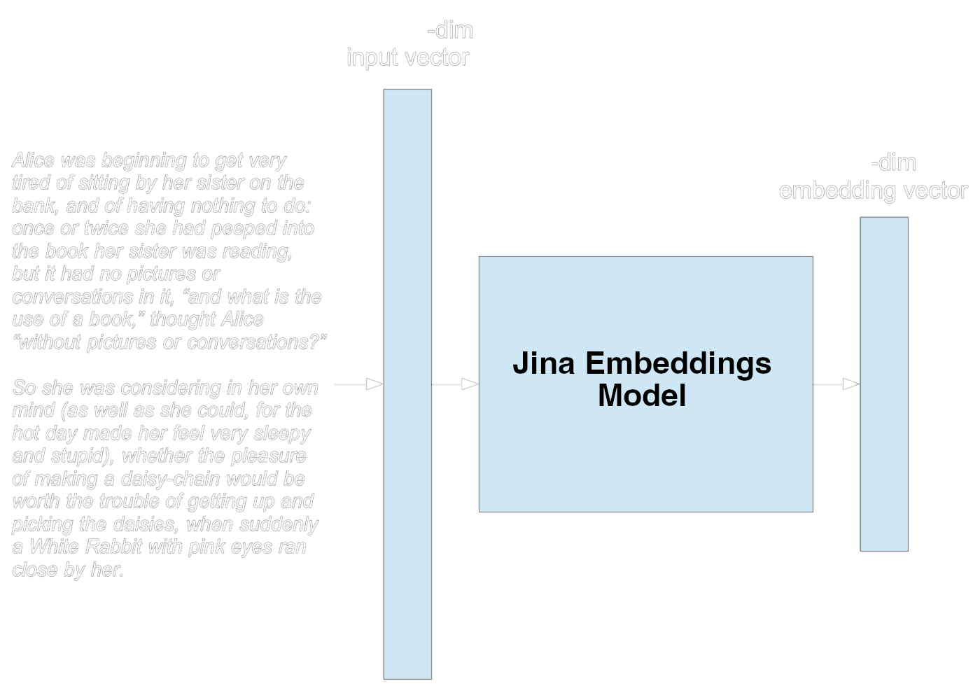
As a concrete example, the Jina Embeddings 2 models represent each token with a 512-dimension vector and can accept a maximum of 8192 tokens as input. This AI model, therefore, has an input vector size of 512x8192 or 4,194,304 dimensions. If the input text is less than 8192 tokens long, the rest of the input vector is set to zeros. If longer, it’s truncated.

The model outputs a 512-dimension embedding vector to represent the input text.

As a developer or user, you don’t have to deal directly with any of these complexities. They are hidden from you by software libraries and web APIs that make using embeddings very straightforward. To transform a text into an embedding can involve as little as one line of code:

curl <https://api.jina.ai/v1/embeddings> \\
  -H "Content-Type: application/json" \\
  -H "Authorization: Bearer jina_xxxxxxxxxxxxxxxxxxxxxxxxxxxxxxx" \\
  -d '{
    "input": ["Your text string goes here", "You can send multiple texts"],
    "model": "jina-embeddings-v2-base-en"
  }'

Go to the Jina Embeddings page to get a token and see code snippets for how to get embeddings in your development environment and programming language.

Embedding API

Top-performing, 8192-token length, $100 for 1.25B tokens, seamless OpenAI alternative, free trial

Embeddings: The Heart of AI

Practically all models have an embedding layer in them, even if it's only implicit, and most AI projects can be built on top of embedding models. That's why good embeddings are so important to the effective use of AI technologies.

This series of articles is designed to demystify embeddings so that you can better understand and oversee the introduction of this technology in your business. Read the first installment here. Next, we will dive further into this technology, and provide hands-on tutorials with code you can use in your own projects.

Jina AI is committed to providing you with tools and help for creating, optimizing, evaluating, and implementing embedding models for your enterprise. We’re here to help you navigate the new world of business AI. Contact us via our website or join our community on Discord to get started.

Jina AI - Your Portal to Multimodal AI

Jina AI offers powerful multimodal AI solutions for everyday users, developers, and scalable enterprise solutions. We aim to democratize access to the limitless potential of AI-generated creativity and innovation, empowering individuals and businesses alike.

Your Portal to Multimodal AI

Join the Jina AI Discord Server!

Check out the Jina AI community on Discord - hang out with 3602 other members and enjoy free voice and text chat.

Discord