Scaling Test-Time Compute For Embedding Models
Better results scale with compute—more on learning, more on search. A good pretrained model takes you far, but test-time compute takes you further. It's time to recognize this paradigm of test-time compute, even for embedding models.

Since OpenAI's release of the O1 model, one of the most discussed topics in the AI community has been scaling test-time compute. This refers to using more computational resources during inference—the phase where an LLM generates outputs—rather than during pre-training or post-training. A well-known example is the Chain-of-Thought (CoT) multi-step reasoning, which enables models to perform more extensive internal deliberations, such as evaluating multiple potential answers, deeper planning, self-reflection before arriving at a final response. Let the model think more rather than train more—this strategy improves answer quality, especially in complex reasoning tasks. Alibaba's recently released QwQ-32B-Preview model follows this trend of improving AI reasoning via scaling test-time compute.
When using OpenAI's O1 model, users can clearly notice that multi-step inference requires additional time as the model constructs reasoning chains to solve problems.
At Jina AI, we focus more on embeddings and rerankers than on LLMs, so for us it's natural to consider scaling test-time compute in this context: Can CoT be applied to embedding models as well? While it might not seem intuitive at first, this article explores a novel perspective and demonstrates how scaling test-time compute can be applied to jina-clip to classify out-of-distribution (OOD) images—solving tasks that would otherwise be impossible.

Case Study

Our experiment focused on Pokemon classification using the TheFusion21/PokemonCards dataset, which contains thousands of Pokemon trading card images. The task is image classification where the input is a cropped Pokemon card artwork (with all text/descriptions removed) and the output is the correct Pokemon name from a predefined set of names. This task presents a particularly interesting challenge for CLIP embedding models because:
- Pokemon names and visuals represent niche, out-of-distribution concepts for the model, making direct classification challenging
- Each Pokemon has clear visual traits that can be decomposed into basic elements (shapes, colors, poses) that CLIP might better understand
- The card artwork provides a consistent visual format while introducing complexity through varying backgrounds, poses, and artistic styles
- The task requires integrating multiple visual features simultaneously, similar to complex reasoning chains in language models

Absol G, Aerodactyl, Weedle, Caterpie, Azumarill, Bulbasaur, Venusaur, Absol, Aggron, Beedrill δ, Alakazam, Ampharos, Dratini, Ampharos, Ampharos, Arcanine, Blaine's Moltres, Aerodactyl, Celebi & Venusaur-GX, Caterpie]Baseline
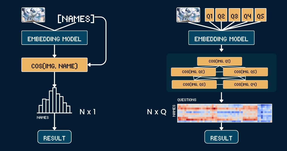
The baseline approach uses a simple direct comparison between Pokemon card artwork and names. First, we crop each Pokemon card image to remove all textual information (header, footer, description) to prevent any trivial guesses from the CLIP model due to Pokemon names appearing in those texts. Then we encode both the cropped images and the Pokemon names using the jina-clip-v1 and jina-clip-v2 model to get their respective embeddings. The classification is done by computing cosine similarity between these image and text embeddings - each image is matched to the name that has the highest similarity score. This creates a straightforward one-to-one matching between visual card artwork and Pokémon names, without any additional context or attribute information. The pseudo code below summarizes the baseline method.
# Preprocessing
cropped_images = [crop_artwork(img) for img in pokemon_cards]  # Remove text, keep only art
pokemon_names = ["Absol", "Aerodactyl", ...]  # Raw Pokemon names

# Get embeddings using jina-clip-v1
image_embeddings = model.encode_image(cropped_images)
text_embeddings = model.encode_text(pokemon_names)

# Classification by cosine similarity
similarities = cosine_similarity(image_embeddings, text_embeddings)
predicted_names = [pokemon_names[argmax(sim)] for sim in similarities]

# Evaluate
accuracy = mean(predicted_names == ground_truth_names)
Chain-of-Thought for Classification

Instead of directly matching images to names, we decompose Pokemon recognition into a structured system of visual attributes. We define five key attribute groups: dominant color (e.g., "white", "blue"), primary form (e.g., "a wolf", "a winged reptile"), key trait (e.g., "a single white horn", "large wings"), body shape (e.g., "wolf-like on four legs", "winged and slender"), and background scene (e.g., "outer space", "green forest").
For each attribute group, we create specific text prompts (e.g., "This Pokémon's body is mainly {} in color") paired with relevant options. We then use the model to compute similarity scores between the image and each attribute option. These scores are converted to probabilities using softmax to get a more calibrated measure of confidence.
The full Chain of Thought (CoT) structure consists of two parts: classification_groups which describes groups of prompts, and pokemon_rules which defines which attribute options each Pokemon should match. For instance, Absol should match with "white" for color and "wolf-like" for form. The full CoT is shown below (we shall explain how this is constructed later):
pokemon_system = {
    "classification_cot": {
        "dominant_color": {
            "prompt": "This Pokémon’s body is mainly {} in color.",
            "options": [
                "white",    # Absol, Absol G
                "gray",     # Aggron
                "brown",    # Aerodactyl, Weedle, Beedrill δ
                "blue",     # Azumarill
                "green",    # Bulbasaur, Venusaur, Celebi&Venu, Caterpie
                "yellow",   # Alakazam, Ampharos
                "red",      # Blaine's Moltres
                "orange",   # Arcanine
                "light blue"# Dratini
            ]
        },
        "primary_form": {
            "prompt": "It looks like {}.",
            "options": [
                "a wolf",         # Absol, Absol G
                "an armored dinosaur",  # Aggron
                "a winged reptile",     # Aerodactyl
                "a rabbit-like creature", # Azumarill
                "a toad-like creature",   # Bulbasaur, Venusaur, Celebi&Venu
                "a caterpillar larva",    # Weedle, Caterpie
                "a wasp-like insect",     # Beedrill δ
                "a fox-like humanoid",     # Alakazam
                "a sheep-like biped",      # Ampharos
                "a dog-like beast",        # Arcanine
                "a flaming bird",          # Blaine’s Moltres
                "a serpentine dragon"      # Dratini
            ]
        },
        "key_trait": {
            "prompt": "Its most notable feature is {}.",
            "options": [
                "a single white horn", # Absol, Absol G
                "metal armor plates",  # Aggron
                "large wings",         # Aerodactyl, Beedrill δ
                "rabbit ears",         # Azumarill
                "a green plant bulb",  # Bulbasaur, Venusaur, Celebi&Venu
                "a small red spike",   # Weedle
                "big green eyes",      # Caterpie
                "a mustache and spoons", # Alakazam
                "a glowing tail orb",  # Ampharos
                "a fiery mane",        # Arcanine
                "flaming wings",       # Blaine's Moltres
                "a tiny white horn on head" # Dratini
            ]
        },
        "body_shape": {
            "prompt": "The body shape can be described as {}.",
            "options": [
                "wolf-like on four legs",   # Absol, Absol G
                "bulky and armored",        # Aggron
                "winged and slender",       # Aerodactyl, Beedrill δ
                "round and plump",          # Azumarill
                "sturdy and four-legged",   # Bulbasaur, Venusaur, Celebi&Venu
                "long and worm-like",       # Weedle, Caterpie
                "upright and humanoid",     # Alakazam, Ampharos
                "furry and canine",         # Arcanine
                "bird-like with flames",    # Blaine's Moltres
                "serpentine"                # Dratini
            ]
        },
        "background_scene": {
            "prompt": "The background looks like {}.",
            "options": [
                "outer space",      # Absol G, Beedrill δ
                "green forest",     # Azumarill, Bulbasaur, Venusaur, Weedle, Caterpie, Celebi&Venu
                "a rocky battlefield", # Absol, Aggron, Aerodactyl
                "a purple psychic room", # Alakazam
                "a sunny field",     # Ampharos
                "volcanic ground",   # Arcanine
                "a red sky with embers", # Blaine's Moltres
                "a calm blue lake"   # Dratini
            ]
        }
    },

    "pokemon_rules": {
        "Absol": {
            "dominant_color": 0,
            "primary_form": 0,
            "key_trait": 0,
            "body_shape": 0,
            "background_scene": 2
        },
        "Absol G": {
            "dominant_color": 0,
            "primary_form": 0,
            "key_trait": 0,
            "body_shape": 0,
            "background_scene": 0
        },
        // ...
    }
}
The final classification combines these attribute probabilities - instead of a single similarity comparison, we're now making multiple structured comparisons and aggregating their probabilities to make a more informed decision.
# Classification process
def classify_pokemon(image):
   # Generate all text prompts
   all_prompts = []
   for group in classification_cot:
       for option in group["options"]:
           prompt = group["prompt"].format(option)
           all_prompts.append(prompt)

   # Get embeddings and similarities
   image_embedding = model.encode_image(image)
   text_embeddings = model.encode_text(all_prompts)
   similarities = cosine_similarity(image_embedding, text_embeddings)

   # Convert to probabilities per attribute group
   probabilities = {}
   for group_name, group_sims in group_similarities:
       probabilities[group_name] = softmax(group_sims)

   # Score each Pokemon based on matching attributes
   scores = {}
   for pokemon, rules in pokemon_rules.items():
       score = 0
       for group, target_idx in rules.items():
           score += probabilities[group][target_idx]
       scores[pokemon] = score

   return max(scores, key=scores.get)
Complexity Analysis
Let's say we want to classify an image into one of N Pokémon names. The baseline approach requires computing N text embeddings (one for each Pokémon name). In contrast, our scaled test-time compute approach requires computing Q text embeddings, where Q is the total number of question-option combinations across all questions. Both methods require computing one image embedding and performing a final classification step, so we exclude these common operations from our comparison. In this case study, ourN=13 and Q=52, which means we our CoT classification takes 4x longer inference time than the baseline.
In an extreme case where Q = N, our approach would essentially reduce to the baseline. However, the key to effectively scaling test-time compute is to:
- Construct carefully chosen questions that increase
Q - Ensure each question provides distinct, informative clues about the final answer
- Design questions to be as orthogonal as possible to maximize their joint information gain.
This approach is analogous to the "Twenty Questions" game, where each question is strategically chosen to narrow down the possible answers effectively.
Evaluation
Our evaluation was conducted on 117 test images spanning 13 different Pokémon classes. And the result is following:
| Approach | jina-clip-v1 | jina-clip-v2 |
|---|---|---|
| Baseline | 31.36% | 16.10% |
| CoT | 46.61% | 38.14% |
| Improvement | +15.25% | +22.04% |
One can see that the same CoT classification offers significant improvements for both models (+15.25% and +22.04% respectively) on this uncommon or OOD task. This also suggests that once the pokemon_system is constructed, the same CoT system can be effectively transferred across different models; and there is no fine-tuning or post-training required.
How Does It Work Again?
Let's recap: We started with fixed pretrained embedding models that couldn't handle zero-shot OOD problems. Then we set up a classification tree, and suddenly they could. What's the secret sauce? Is it the weak learner ensemble idea, as in classic machine learning?
It's worth highlighting that our embedding model's upgrade from "can't" to "can" isn't due to the ensemble itself, but rather due to the external domain knowledge in that classification tree. One can repeatedly apply zero-shot classification on thousands of questions, but if answering them doesn't contribute to the final answer, then it's pointless. Think about the "20 Questions" game, where you want to narrow down the solution space after each question. Hence, this external knowledge or thought process is much more crucial - in our example, it's about how the Pokémon system is constructed. This expert knowledge can come from either humans or an LLM.
Constructing pokemon_system Effectively
The effectiveness of our scaled test-time compute approach heavily depends on how well we construct the pokemon_system. There are different approaches to building this system, from manual to fully automated.
Manual Construction
The most straightforward approach is to manually analyze the Pokemon dataset and create attribute groups, prompts, and rules. A domain expert would need to identify key visual attributes such as color, form, and distinctive features. They would then write natural language prompts for each attribute, enumerate possible options for each attribute group, and map each Pokemon to its correct attribute options. While this provides high-quality rules, it's time-consuming and doesn't scale well to larger N.
LLM-Assisted Construction
We can leverage LLMs to accelerate this process by prompting them to generate the classification system. A well-structured prompt would request attribute groups based on visual characteristics, natural language prompt templates, comprehensive and mutually exclusive options, and mapping rules for each Pokemon. The LLM can quickly generate a first draft, though its output may need verification.
I need help creating a structured system for Pokemon classification. For each Pokemon in this list: [Absol, Aerodactyl, Weedle, Caterpie, Azumarill, ...], create a classification system with:

1. Classification groups that cover these visual attributes:
   - Dominant color of the Pokemon
   - What type of creature it appears to be (primary form)
   - Its most distinctive visual feature
   - Overall body shape
   - What kind of background/environment it's typically shown in

2. For each group:
   - Create a natural language prompt template using "{}" for the option
   - List all possible options that could apply to these Pokemon
   - Make sure options are mutually exclusive and comprehensive

3. Create rules that map each Pokemon to exactly one option per attribute group, using indices to reference the options

Please output this as a Python dictionary with two main components:
- "classification_groups": containing prompts and options for each attribute
- "pokemon_rules": mapping each Pokemon to its correct attribute indices

Example format:
{
    "classification_groups": {
        "dominant_color": {
            "prompt": "This Pokemon's body is mainly {} in color",
            "options": ["white", "gray", ...]
        },
        ...
    },
    "pokemon_rules": {
        "Absol": {
            "dominant_color": 0,  # index for "white"
            ...
        },
        ...
    }
}
A more robust approach combines LLM generation with human validation. First, the LLM generates an initial system. Then, human experts review and correct attribute groupings, option completeness, and rule accuracy. The LLM refines the system based on this feedback, and the process iterates until satisfactory quality is achieved. This approach balances efficiency with accuracy.
Automated Construction with DSPy
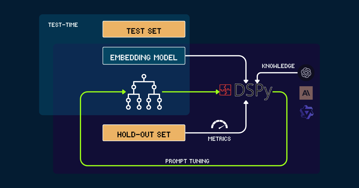
For a fully automated approach, we can use DSPy to iteratively optimize pokemon_system. The process begins with a simple pokemon_system written either manually or by LLMs as an initial prompt. Each version is evaluated on a hold-out set, using accuracy as a feedback signal for DSPy. Based on this performance, optimized prompts (i.e., new versions of pokemon_system) are generated. This cycle repeats until convergence, and during the entire process, the embedding model remains completely fixed.

pokemon_system CoT design; the tuning process needs to be done only once for each task.Why Scale Test-Time Compute for Embedding Models?
Because scaling pretraining eventually becomes economically intractable.
Since the release of the Jina embeddings suite—including jina-embeddings-v1, v2, v3, jina-clip-v1, v2, and jina-ColBERT-v1, v2—each model upgrade through scaled pretraining has come with more costs. For example, our first model, jina-embeddings-v1, released in June 2023 with 110M parameters. Training it back then cost between 5,000 and 20,000 USD depending how you measure. With jina-embeddings-v3, improvements are significant, but they primarily stem from the increased resources invested. The cost trajectory for frontier models has gone from thousands to tens of thousands of dollars and, for larger AI companies, even hundreds of millions today. While throwing more money, resources, and data at pretraining yields better models, the marginal returns eventually make further scaling economically unsustainable.

On the other hand, modern embedding models are becoming increasingly powerful: multilingual, multitask, multimodal, and capable of strong zero-shot and instruction-following performance. This versatility leaves big room for algorithmic improvements and scaling test-time compute.
The question then becomes: what is the cost users are willing to pay for a query they care deeply about? If tolerating longer inference times for fixed pretraining models significantly improves the quality of the results, many would find that worthwhile. In our view, there's substantial untapped potential in scaling test-time compute for embedding models. This represents a shift from merely increasing model size during training to enhancing computational effort during the inference phase to achieve better performance.
Conclusion
Our case study on test-time compute of jina-clip-v1/v2 shows several key findings:
- We achieved better performance on uncommon or out-of-distribution (OOD) data without any fine-tuning or post-training on embeddings.
- The system made more nuanced distinctions by iteratively refining similarity searches and classification criteria.
- By incorporating dynamic prompt adjustments and iterative reasoning, we transformed the embedding model's inference process from a single query into a more sophisticated chain of thought.
This case study merely scratches the surface of what's possible with test-time compute. There remains substantial room for scaling algorithmically. For example, we could develop methods to iteratively select questions that most efficiently narrow down the answer space, similar to the optimal strategy in the "Twenty Questions" game. By scaling test-time compute, we can push embedding models beyond their current limitations and enable them to tackle more complex, nuanced tasks that once seemed out of reach.

