Text-Image Global Contrastive Alignment and Token-Patch Local Alignment
CLIP can visualize token-patch similarities, however, it’s more of a post-hoc interpretability trick than a robust or official "attention" from the model. Here's why.

While experimenting with ColPali-style models, one of our engineers created a visualization using our recently released jina-clip-v2 model. He mapped the similarity between token embeddings and patch embeddings for given image-text pairs, creating heatmap overlays that produced some intriguing visual insights.
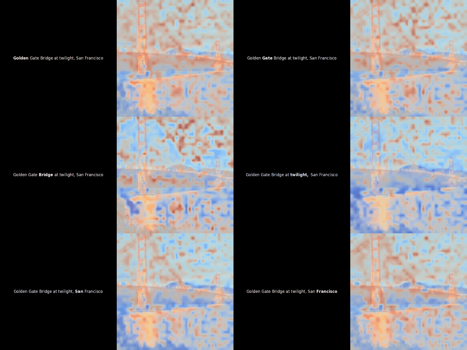
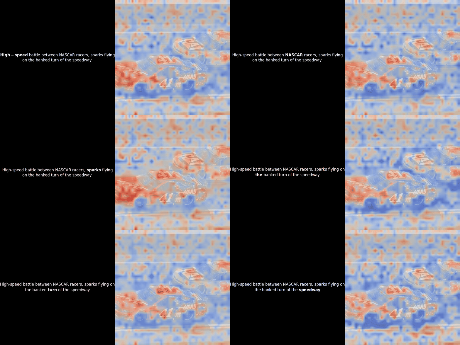
Unfortunately, this is just a heuristic visualization - not an explicit or guaranteed mechanism. While CLIP-like global contrastive alignment can (and often does) incidentally create rough local alignments between patches and tokens, this is an unintended side effect rather than a deliberate objective of the model. Let me explain why.
Understand the Code

Let's break down what the code is doing at a high level. Note that jina-clip-v2 doesn't actually expose any API for accessing token-level or patch-level embeddings by default - this visualization required some post-hoc patching to make it work.
Compute word-level embeddings
By setting model.text_model.output_tokens = True, calling text_model(x=...,)[1] will return a (batch_size, seq_len, embed_dim) second element for the token embeddings. So it takes an input sentence, tokenizes it with the Jina CLIP tokenizer, and then groups subword tokens back into “words” by averaging the corresponding token embeddings. It detects the start of a new word by checking if the token string begins with the _ character (typical in SentencePiece-based tokenizers). It produces a list of word-level embeddings and a list of words (so that “Dog” is one embedding, “and” is one embedding, etc.).
Compute patch-level embeddings
For image tower, vision_model(..., return_all_features=True) will return (batch_size, n_patches+1, embed_dim), where the first token is the [CLS] token. From that, the code extracts the embeddings for each patch (i.e., the vision transformer’s patch tokens). It then reshapes these patch embeddings into a 2D grid, patch_side × patch_side, which is then upsampled to match the original image resolution.
Visualize word-patch similarity
The similarity calculation and the subsequent heatmap generation are standard “post-hoc” interpretability techniques: you pick a text embedding, compute cosine similarity with every patch embedding, and then generates a heatmap showing which patches have the highest similarity to that specific token embedding. Finally, it cycles through each token in the sentence, highlights that token in bold on the left, and overlays the similarity-based heatmap on the original image on the right. All frames are compiled into an animated GIF.
Is It Meaningful Explainability?
From a pure code standpoint, yes, the logic is coherent and will produce a heatmap for each token. You’ll get a series of frames that highlight patch similarities, so the script “does what it says on the tin.”
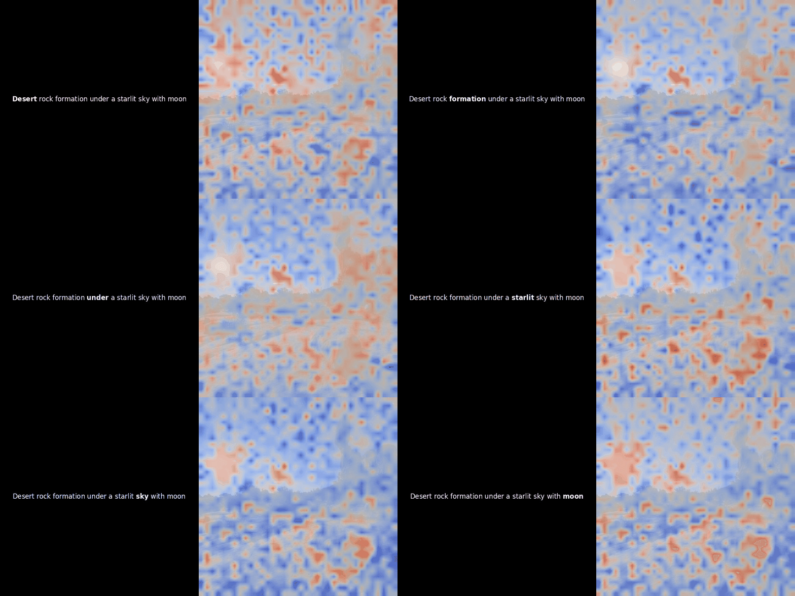
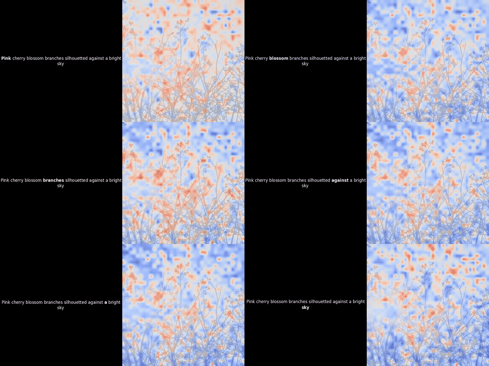
Looking at the examples above, we see that words like moon and branches appear to align well with their corresponding visual patches in the original image. But here's the key question: is this meaningful alignment, or are we just seeing a fortunate coincidence?
This is a deeper question. To understand the caveats, recall how CLIP is trained:

- CLIP uses global contrastive alignment between an entire image and an entire piece of text. During training, the image encoder produces a single vector (pooled representation), and the text encoder produces another single vector; CLIP is trained so that these match for matching text-image pairs and mismatch otherwise.
- There is no explicit supervision at the level of ‘patch X corresponds to token Y’. The model is not directly trained to highlight “this region of the image is the dog, that region is the cat,” etc. Instead, it is taught that the entire image representation should match the entire text representation.
- Because CLIP’s architecture is a Vision Transformer on the image side and a text transformer on the text side—both forming separate encoders—there is no cross-attention module that natively aligns patches to tokens. Instead, you get purely self-attention in each tower, plus a final projection for the global image or text embeddings.
In short, this is a heuristic visualization. The fact that any given patch embedding might be close or far from a particular token embedding is somewhat emergent. It’s more of a post-hoc interpretability trick than a robust or official “attention” from the model.
Why Might Local Alignment Emerge?
So why might we sometimes spot word-patch level local alignments? Here's the thing: even though CLIP is trained on a global image-text contrastive objective, it still uses self-attention (in ViT-based image encoders) and transformer layers (for text). Within these self-attention layers, different parts of image representations can interact with each other, just as words do in text representations. Through training on massive image-text datasets, the model naturally develops internal latent structures that help it match overall images to their corresponding text descriptions.
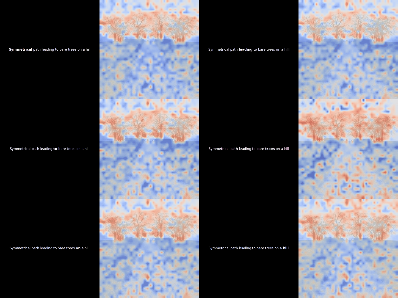
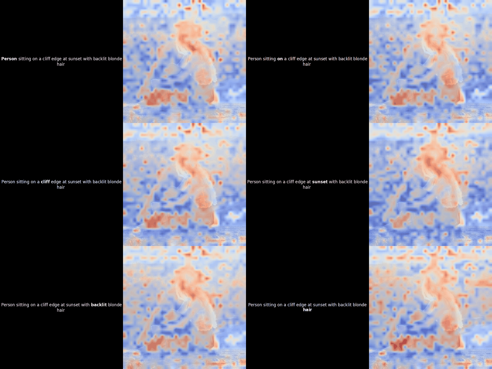
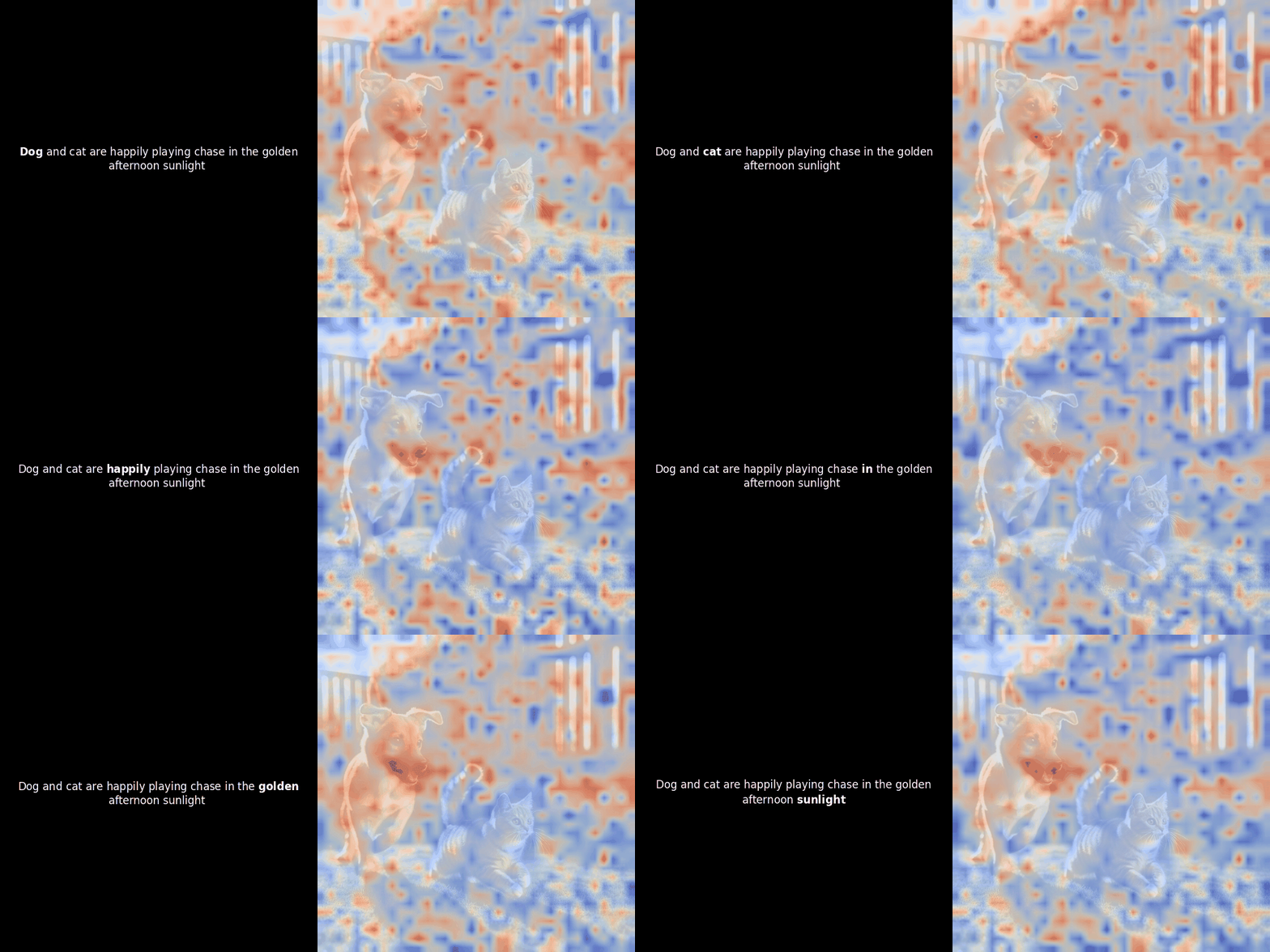
Local alignment can appear in these latent representations for at least two reasons:
- Co-occurrence patterns: If a model sees many images of “dogs” next to many images of “cats” (often labeled or described with those words), it can learn latent features that roughly correspond to these concepts. So the embedding for “dog” might become close to local patches that depict a dog-like shape or texture. This is not explicitly supervised at the patch level, but emerges from repeated association between dog images/text pairs.
- Self-attention: In Vision Transformers, patches attend to each other. Distinctive patches (like a dog’s face) can end up with a consistent latent “signature,” because the model is trying to produce a single globally accurate representation of the entire scene. If that helps minimize the overall contrastive loss, it will get reinforced.
Theoretical Analysis
CLIP's contrastive learning objective aims to maximize the cosine similarity between matching image-text pairs while minimizing it for non-matching pairs. Assume the text and image encoders produce token and patch embeddings respectively:
$$\mathbf{u}_i = \frac{1}{M} \sum_{m=1}^M \mathbf{u}_{i,m}, \quad \mathbf{v}_i = \frac{1}{K} \sum_{k=1}^K \mathbf{v}_{i,k}$$Global similarity can be represented as an aggregate of local similarities:
$$\text{sim}(\mathbf{u}_i, \mathbf{v}_i) = \frac{1}{MK} \sum_{m=1}^M \sum_{k=1}^K \mathbf{u}_{i,m}^\top \mathbf{v}_{i,k}$$When specific token-patch pairs frequently co-occur across the training data, the model reinforces their similarity through cumulative gradient updates:
$$\Delta \mathbf{u}_{m^*} \propto \sum_{c=1}^C \mathbf{v}_{k^*}^{(c)}, \quad \Delta \mathbf{v}_{k^*} \propto \sum_{c=1}^C \mathbf{u}_{m^*}^{(c)}$$, where $C$ is the number of co-occurrences. This leads to $\mathbf{u}_{m^*}^\top \mathbf{v}_{k^*}$ increases significantly, promoting stronger local alignment for these pairs. However, the contrastive loss distributes gradient updates across all token-patch pairs, limiting the strength of updates for any specific pair:
$$\frac{\partial \mathcal{L}}{\partial \mathbf{u}_{m}} \propto -\sum_{k=1}^K \mathbf{v}_k \cdot \left( \frac{\exp(\mathbf{u}^\top \mathbf{v} / \tau)}{\sum_{j=1}^N \exp(\mathbf{u}^\top \mathbf{v}_j / \tau)} \right)$$This prevents significant reinforcement of individual token-patch similarities.
Conclusion
CLIP’s token-patch visualizations capitalizes on an incidental, emergent alignment between text and image representations. This alignment, while intriguing, stems from CLIP’s global contrastive training and lacks the structural robustness required for precise and reliable explainability. The resulting visualizations often exhibit noise and inconsistency, limiting their utility for in-depth interpretative applications.
Late interaction models such as ColBERT and ColPali address these limitations by architecturally embedding explicit, fine-grained alignments between text tokens and image patches. By processing modalities independently and performing targeted similarity computations at a later stage, these models ensure that each text token is meaningfully associated with relevant image regions.


