What Late Chunking Really Is & What It’s Not: Part II

Late Chunking: Contextual Chunk Embeddings Using Long-Context Embedding Models

Many use cases require retrieving smaller portions of text, and dense vector-based retrieval systems often perform better with shorter text segments, as the semantics are less likely to be over-compressed in the embeddings. Consequently, practitioners often split text documents into smaller chunks and encode them separately. However, chunk embeddings created in this way can lose contextual information from surrounding chunks, resulting in sub-optimal representations. In this paper, we introduce a novel method called late chunking, which leverages long context embedding models to first embed all tokens of the long text, with chunking applied after the transformer model and just before mean pooling - hence the term late in its naming. The resulting chunk embeddings capture the full contextual information, leading to superior results across various retrieval tasks. The method is generic enough to be applied to a wide range of long-context embedding models and works without additional training. To further increase the effectiveness of late chunking, we propose a dedicated fine-tuning approach for embedding models.

arXiv.orgMichael Günther

Chunking a long document has two issues: first, determining the breakpoints—i.e., how to segment the document. You might consider fixed token lengths, a fixed number of sentences, or more advanced techniques like regex or semantic segmentation models. Accurate chunk boundaries not only improve the readability of the search results, but also ensure that the chunks fed to an LLM in a RAG system is precise and sufficient—no more, no less.

The second issue is the loss of context within each chunk. Once the document is segmented, most people’s next logical step is to embed each chunk separately in a batch process. However, this leads to a loss of global context from the original document. Many previous works have tackled the first issue first, arguing that better boundary detection improves semantic representation. For example, "semantic chunking" groups sentences with high cosine similarity in the embedding space to minimize the disruption of semantic units.

From our POV, these two issues are almost orthogonal and can be tackled separately. If we had to prioritize, we’d say the 2nd issue is more critical.

Late Chunking for Context Loss

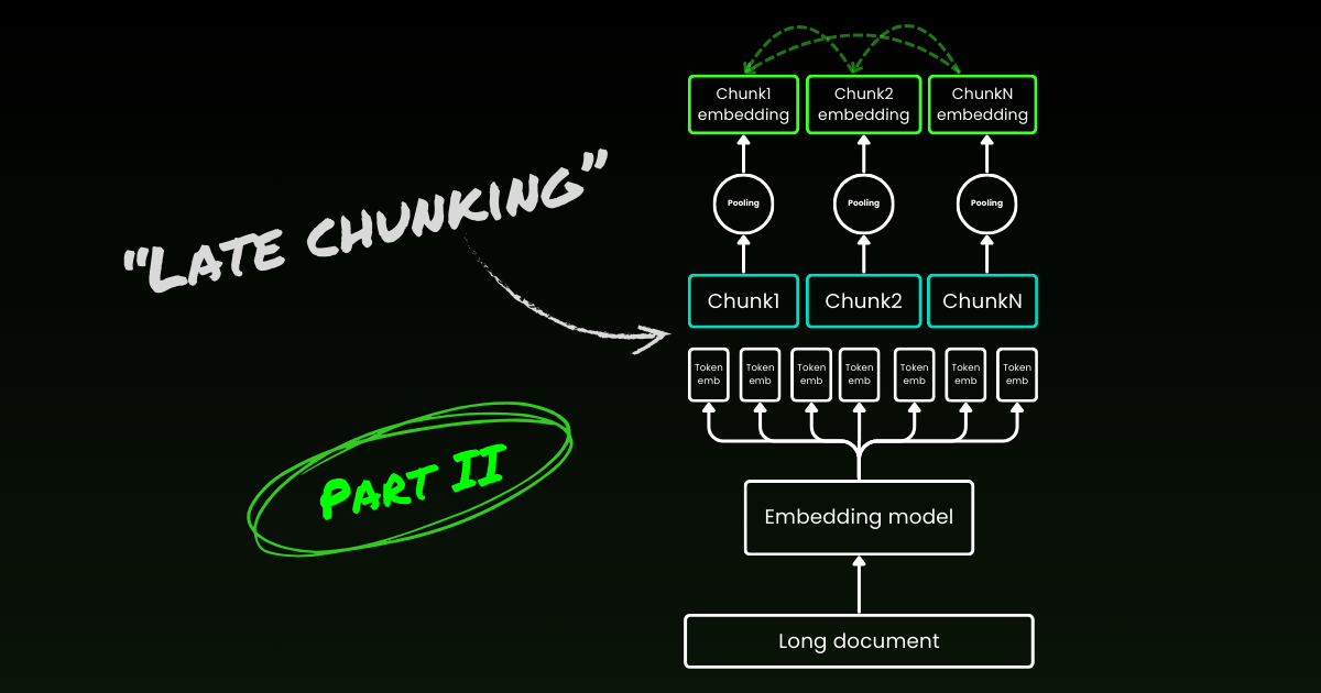
Late chunking starts by addressing the second issue: loss of context. It’s not about finding the ideal breakpoints or semantic boundaries. You still need to use regex, heuristics, or other techniques to divide a long document into small chunks. But instead of embedding each chunk as soon as it's segmented, late chunking first encodes the entire document in one context window (for jina-embeddings-v3 it's 8192-token). Then, it follows the boundary cues to apply mean pooling for each chunk—hence the term "late" in late chunking.

Late Chunking is Resilient to Poor Boundary Cues

What's really interesting is that experiments show late chunking eliminates the need for perfect semantic boundaries, which partially addresses the first issue mentioned above. In fact, late chunking applied to fixed-token boundaries outperforms naive chunking with semantic boundary cues. Simple segmentation models, like those using fixed-length boundaries, perform on par with advanced boundary detection algorithms when paired with late chunking. We tested three different sizes of embedding models, and results show that all of them consistently benefit from late chunking across all test datasets. That said, the embedding model itself remains the most significant factor in performance—there is not a single instance where a weaker model with late chunking outperforms a stronger model without it.

Note that being resilient to poor boundaries doesn’t mean we can ignore them—they still matter for both human & LLM readability. Here’s how we see it: when optimizing segmentation, i.e. the aforementioned 1st issue, we can focus fully on readability without worrying about semantic/context loss. Late Chunking handles good or bad breakpoints, so readability is all you need to care.

Late Chunking is Bidirectional

Another common misconception about late chunking is that its conditional chunk embeddings rely only on previous chunks without "looking ahead." This is incorrect. The conditional dependency in late chunking is actually bi-directional, not one-directional. This is because the attention matrix in the embedding model—an encoder-only transformer—is fully connected, unlike the masked triangular matrix used in auto-regressive models. Formally, the embedding of chunk $k$, $v_k \sim Q(c_k|D)$, rather than $v_k \sim Q(c_k | c_1, c_2, \cdots, c_{k-1})$, where $Q$ denotes a factorization of the language model. This also explains why late chunking is not dependent on precise boundary placement.

Late Chunking Can Be Trained

Late chunking does not require additional training for embedding models. It can be applied to any long-context embedding models that use mean pooling, making it highly attractive for practitioners. That said, if you're working on tasks like question-answering or query-document retrieval, performance can still be further improved with some fine-tuning. Specifically, the training data consists of tuples containing:

• A query (e.g., a question or search term).
• A document that contains relevant information to answer the query.
• A relevant span within the document, which is the specific chunk of text that directly addresses the query.

The model is trained by pairing queries with their relevant spans, using a contrastive loss function like InfoNCE. This ensures that relevant spans are closely aligned with the query in the embedding space, while unrelated spans are pushed further apart. As a result, the model learns to focus on the most relevant parts of the document when generating chunk embeddings. For more details, please refer to our research paper.

Late Chunking vs. Contextual Retrieval

Introducing Contextual Retrieval

Anthropic is an AI safety and research company that’s working to build reliable, interpretable, and steerable AI systems.

Soon after late chunking was introduced, Anthropic introduced a separate strategy called Contextual Retrieval. Anthropic's method is a brute-force approach to address the issue of lost context, and works as follows:

1. Each chunk is sent to the LLM along with the full document.
2. The LLM adds relevant context to each chunk.
3. This results in richer and more informative embeddings.

In our view, this is essentially context enrichment, where global context is explicitly hardcoded into each chunk using an LLM, which is expensive in terms of cost, time, and storage. Additionally, it’s unclear if this approach is resilient to chunk boundaries, as the LLM relies on accurate and readable chunks to enrich the context effectively. In contrast, late chunking is highly resilient to boundary cues, as demonstrated above. It requires no additional storage since the embedding size remains the same. Despite leveraging the full context length of the embedding model, it is still significantly faster than using an LLM to generate enrichment. In the qualitative study of our research paper, we show that Anthropic's context retrieval performs similarly to late chunking. However, late chunking provides a more low-level, generic, and natural solution by leveraging the inherent mechanics of the encoder-only transformer.

Which Embedding Models Support Late Chunking?

Late chunking isn’t exclusive to jina-embeddings-v3 or v2. It’s a fairly generic approach that can be applied to any long-context embedding model that uses mean pooling. For example, in this post, we show that nomic-v1 supports it too. We warmly welcome all embedding providers to implement support for late chunking in their solutions.

As a model user, when evaluating a new embedding model or API, you can follow these steps to check if it might support late chunking:

1. Single Output: Does the model/API give you just one final embedding per sentence instead of token-level embeddings? If yes, then it likely can’t support late chunking (especially for those web APIs).
2. Long-Context Support: Does the model/API handle contexts of at least 8192 tokens? If not, late chunking won’t be applicable—or more precisely, it doesn’t make sense to adapt late chunking for a short-context model. If yes, ensure it actually performs well with long contexts, not just claims to support them. You can usually find this info in the model’s technical report, such as evaluations on LongMTEB or other long-context benchmarks.
3. Mean Pooling: For self-hosted models or APIs that provide token-level embeddings before pooling, check if the default pooling method is mean pooling. Models using CLS or max pooling aren’t compatible with late chunking.

In summary, if an embedding model supports long-context and uses mean pooling by default, it can easily support late chunking. Check out our GitHub repo for implementation details and further discussion.

Conclusion

So, what is late chunking? Late chunking is a straightforward method for generating chunk embeddings using long-context embedding models. It’s fast, resilient to boundary cues, and highly effective. It’s not a heuristic or over-engineering—it's a thoughtful design rooted in a deep understanding of the transformer mechanism.

Today, the hype surrounding LLMs is undeniable. In many cases, problems that could be efficiently tackled by smaller models like BERT are instead handed off to LLMs, driven by the allure of larger, more complex solutions. It’s no surprise that big LLM providers push for greater adoption of their models, while embedding providers advocate for embeddings — both are playing to their commercial strengths. But in the end, it’s not about the hype, it's about action, about what truly works. Let the community, the industry, and, most importantly, time reveal which approach is truly leaner, more efficient, and built to last.

Be sure to read our research paper, and we encourage you to benchmark late chunking in various scenarios and share your feedback with us.